OpenSA

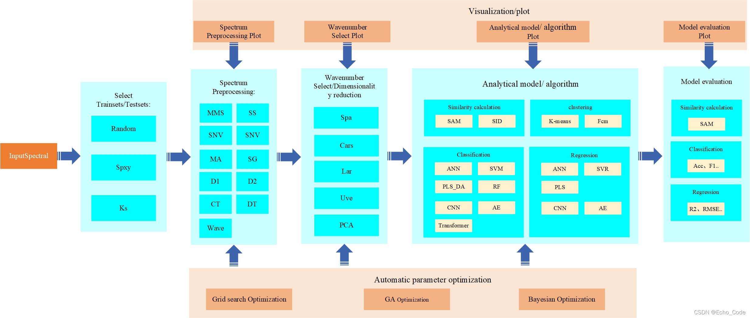
Aiming at the common training datsets split, spectrum preprocessing, wavelength select and calibration models algorithm involved in the spectral analysis process, a complete algorithm library is established, which is named opensa (openspectrum analysis).

系列文章目录

“光晰本质，谱见不同”，光谱作为物质的指纹，被广泛应用于成分分析中。伴随微型光谱仪/光谱成像仪的发展与普及，基于光谱的分析技术将不只停留于工业和实验室，即将走入生活，实现万物感知，见微知著。本系列文章致力于光谱分析技术的科普和应用。

@TOC

前言

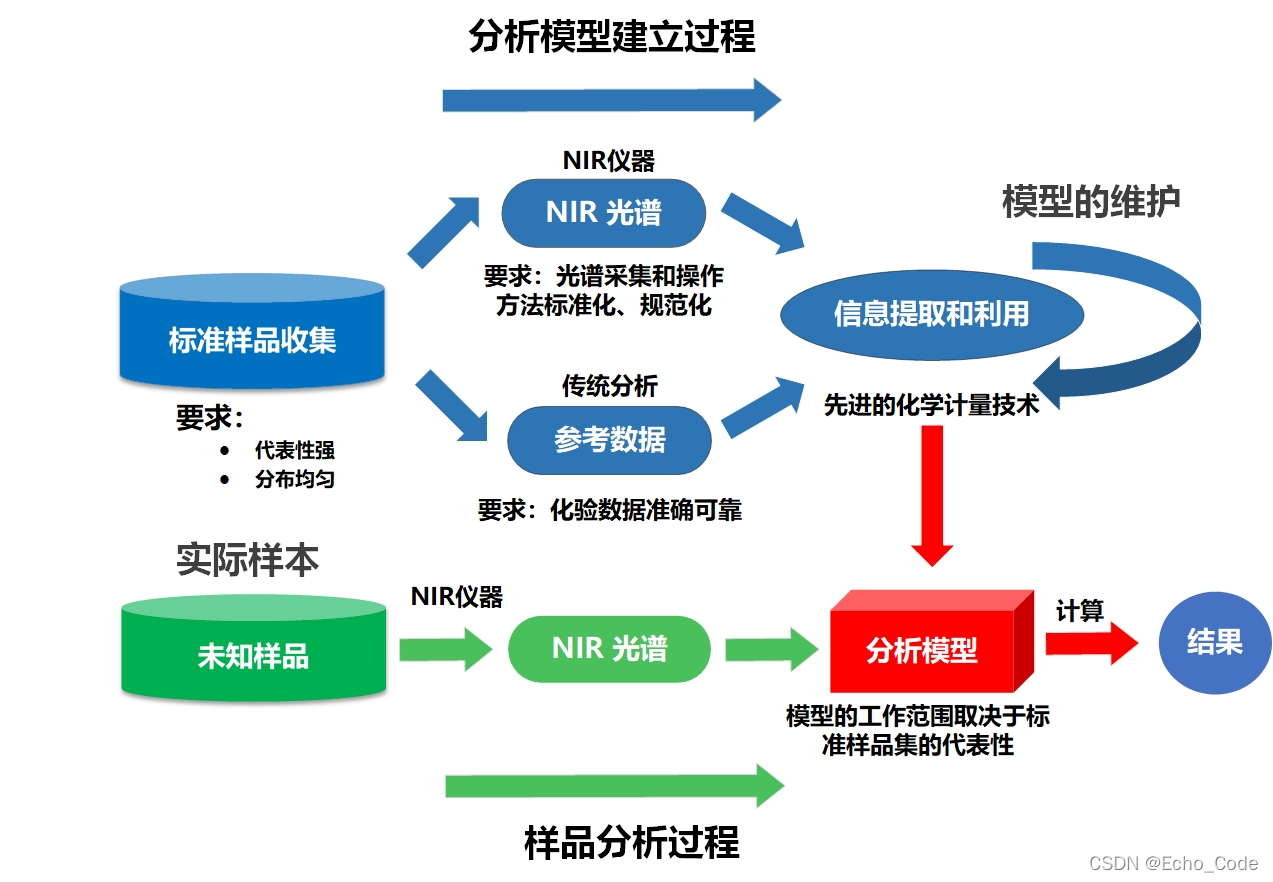
典型的光谱分析模型(以近红外光谱作为示意，可见光、中远红外、荧光、拉曼、高光谱等分析流程亦相似)建立流程如下所示，在建立过程中，需要使用算法对训练样本进行选择，然后使用预处理算法对光谱进行预处理，或对光谱的特征进行提取，再构建校正模型实现定量分析，最后针对不同测量仪器或环境，进行模型转移或传递。因此训练样本的选择、光谱的预处理、波长筛选、校正模型、模型传递以及上述算法的参数都影响着模型的应用效果。

针对光谱分析流程所涉及的常见的训练样本的划分、光谱的预处理、波长筛选、校正模型算法建立了完整的算法库，名为OpenSA(OpenSpectrumAnalysis)。整套算法库的架构如下所示。样本划分模块提供随机划分、SPXY划分、KS划分三种数据集划分方法，光谱预处理模块提供常见光谱预处理，波长筛选模块提供Spa、Cars、Lars、Uve、Pca等特征降维方法，分析模块由光谱相似度计算、聚类、分类(定性分析)、回归(定量分析)构建，光谱相似度子模块计算提供SAM、SID、MSSIM、MPSNR等相似计算方法，聚类子模块提供KMeans、FCM等聚类方法，分类子模块提供ANN、SVM、PLS_DA、RF等经典化学计量学方法，亦提供CNN、AE、Transformer等前沿深度学习方法，回归子模块提供ANN、SVR、PLS等经典化学计量学定量分析方法，亦提供CNN、AE、Transformer等前沿深度学习定量分析方法。模型评估模块提供常见的评价指标，用于模型评估。自动参数优化模块用于自动进行最佳的模型设置参数寻找，提供网格搜索、遗传算法、贝叶斯概率三种最优参数寻找方法。可视化模块提供全程的分析可视化，可为科研绘图，模型选择提供视觉信息。可通过几行代码快速实现完整的光谱分析及应用（注: 自动参数优化模块和可视化模块暂不开源，等毕业后再说)

本篇针对OpenSA的光谱预处理模块进行代码开源和使用示意。

一、光谱数据读入

提供两个开源数据作为实列，一个为公开定量分析数据集，一个为公开定性分析数据集，本章仅以公开定量分析数据集作为演示。

1.1 光谱数据读入

# 分别使用一个回归、一个分类的公开数据集做为example
def LoadNirtest(type):

    if type == "Rgs":
        CDataPath1 = './/Data//Rgs//Cdata1.csv'
        VDataPath1 = './/Data//Rgs//Vdata1.csv'
        TDataPath1 = './/Data//Rgs//Tdata1.csv'

        Cdata1 = np.loadtxt(open(CDataPath1, 'rb'), dtype=np.float64, delimiter=',', skiprows=0)
        Vdata1 = np.loadtxt(open(VDataPath1, 'rb'), dtype=np.float64, delimiter=',', skiprows=0)
        Tdata1 = np.loadtxt(open(TDataPath1, 'rb'), dtype=np.float64, delimiter=',', skiprows=0)

        Nirdata1 = np.concatenate((Cdata1, Vdata1))
        Nirdata = np.concatenate((Nirdata1, Tdata1))
        data = Nirdata[:, :-4]
        label = Nirdata[:, -1]

    elif type == "Cls":
        path = './/Data//Cls//table.csv'
        Nirdata = np.loadtxt(open(path, 'rb'), dtype=np.float64, delimiter=',', skiprows=0)
        data = Nirdata[:, :-1]
        label = Nirdata[:, -1]

    return data, label

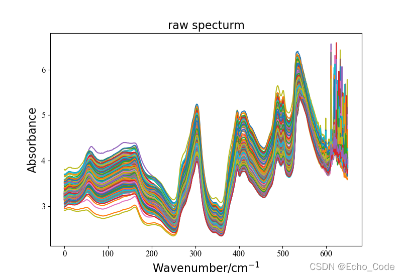
1.2 光谱可视化

    #载入原始数据并可视化
    data, label = LoadNirtest('Rgs')
    plotspc(data, "raw specturm")

采用的开源光谱如图所示:

二、光谱预处理

2.1 光谱预处理模块

将常见的光谱进行了封装，使用者仅需要改变名字，即可选择对应的光谱分析，下面是光谱预处理模块的核心代码

"""
    -*- coding: utf-8 -*-
    @Time   :2022/04/12 17:10
    @Author : Pengyou FU
    @blogs  : https://blog.csdn.net/Echo_Code?spm=1000.2115.3001.5343
    @github :
    @WeChat : Fu_siry
    @License：

"""
import numpy as np
from scipy import signal
from sklearn.linear_model import LinearRegression
from sklearn.preprocessing import MinMaxScaler, StandardScaler
from copy import deepcopy
import pandas as pd
import pywt


# 最大最小值归一化
def MMS(data):
    """
       :param data: raw spectrum data, shape (n_samples, n_features)
       :return: data after MinMaxScaler :(n_samples, n_features)
       """
    return MinMaxScaler().fit_transform(data)


# 标准化
def SS(data):
    """
        :param data: raw spectrum data, shape (n_samples, n_features)
       :return: data after StandScaler :(n_samples, n_features)
       """
    return StandardScaler().fit_transform(data)


# 均值中心化
def CT(data):
    """
       :param data: raw spectrum data, shape (n_samples, n_features)
       :return: data after MeanScaler :(n_samples, n_features)
       """
    for i in range(data.shape[0]):
        MEAN = np.mean(data[i])
        data[i] = data[i] - MEAN
    return data


# 标准正态变换
def SNV(data):
    """
        :param data: raw spectrum data, shape (n_samples, n_features)
       :return: data after SNV :(n_samples, n_features)
    """
    m = data.shape[0]
    n = data.shape[1]
    print(m, n)  #
    # 求标准差
    data_std = np.std(data, axis=1)  # 每条光谱的标准差
    # 求平均值
    data_average = np.mean(data, axis=1)  # 每条光谱的平均值
    # SNV计算
    data_snv = [[((data[i][j] - data_average[i]) / data_std[i]) for j in range(n)] for i in range(m)]
    return  data_snv



# 移动平均平滑
def MA(data, WSZ=11):
    """
       :param data: raw spectrum data, shape (n_samples, n_features)
       :param WSZ: int
       :return: data after MA :(n_samples, n_features)
    """

    for i in range(data.shape[0]):
        out0 = np.convolve(data[i], np.ones(WSZ, dtype=int), 'valid') / WSZ # WSZ是窗口宽度，是奇数
        r = np.arange(1, WSZ - 1, 2)
        start = np.cumsum(data[i, :WSZ - 1])[::2] / r
        stop = (np.cumsum(data[i, :-WSZ:-1])[::2] / r)[::-1]
        data[i] = np.concatenate((start, out0, stop))
    return data


# Savitzky-Golay平滑滤波
def SG(data, w=11, p=2):
    """
       :param data: raw spectrum data, shape (n_samples, n_features)
       :param w: int
       :param p: int
       :return: data after SG :(n_samples, n_features)
    """
    return signal.savgol_filter(data, w, p)


# 一阶导数
def D1(data):
    """
       :param data: raw spectrum data, shape (n_samples, n_features)
       :return: data after First derivative :(n_samples, n_features)
    """
    n, p = data.shape
    Di = np.ones((n, p - 1))
    for i in range(n):
        Di[i] = np.diff(data[i])
    return Di


# 二阶导数
def D2(data):
    """
       :param data: raw spectrum data, shape (n_samples, n_features)
       :return: data after second derivative :(n_samples, n_features)
    """
    data = deepcopy(data)
    if isinstance(data, pd.DataFrame):
        data = data.values
    temp2 = (pd.DataFrame(data)).diff(axis=1)
    temp3 = np.delete(temp2.values, 0, axis=1)
    temp4 = (pd.DataFrame(temp3)).diff(axis=1)
    spec_D2 = np.delete(temp4.values, 0, axis=1)
    return spec_D2


# 趋势校正(DT)
def DT(data):
    """
       :param data: raw spectrum data, shape (n_samples, n_features)
       :return: data after DT :(n_samples, n_features)
    """
    lenth = data.shape[1]
    x = np.asarray(range(lenth), dtype=np.float32)
    out = np.array(data)
    l = LinearRegression()
    for i in range(out.shape[0]):
        l.fit(x.reshape(-1, 1), out[i].reshape(-1, 1))
        k = l.coef_
        b = l.intercept_
        for j in range(out.shape[1]):
            out[i][j] = out[i][j] - (j * k + b)

    return out


# 多元散射校正
def MSC(data):
    """
       :param data: raw spectrum data, shape (n_samples, n_features)
       :return: data after MSC :(n_samples, n_features)
    """
    n, p = data.shape
    msc = np.ones((n, p))

    for j in range(n):
        mean = np.mean(data, axis=0)

    # 线性拟合
    for i in range(n):
        y = data[i, :]
        l = LinearRegression()
        l.fit(mean.reshape(-1, 1), y.reshape(-1, 1))
        k = l.coef_
        b = l.intercept_
        msc[i, :] = (y - b) / k
    return msc

# 小波变换
def wave(data):
    """
       :param data: raw spectrum data, shape (n_samples, n_features)
       :return: data after wave :(n_samples, n_features)
    """
    data = deepcopy(data)
    if isinstance(data, pd.DataFrame):
        data = data.values
    def wave_(data):
        w = pywt.Wavelet('db8')  # 选用Daubechies8小波
        maxlev = pywt.dwt_max_level(len(data), w.dec_len)
        coeffs = pywt.wavedec(data, 'db8', level=maxlev)
        threshold = 0.04
        for i in range(1, len(coeffs)):
            coeffs[i] = pywt.threshold(coeffs[i], threshold * max(coeffs[i]))
        datarec = pywt.waverec(coeffs, 'db8')
        return datarec

    tmp = None
    for i in range(data.shape[0]):
        if (i == 0):
            tmp = wave_(data[i])
        else:
            tmp = np.vstack((tmp, wave_(data[i])))

    return tmp

def Preprocessing(method, data):

    if method == "None":
        data = data
    elif method == 'MMS':
        data = MMS(data)
    elif method == 'SS':
        data = SS(data)
    elif method == 'CT':
        data = CT(data)
    elif method == 'SNV':
        data = SNV(data)
    elif method == 'MA':
        data = MA(data)
    elif method == 'SG':
        data = SG(data)
    elif method == 'MSC':
        data = MSC(data)
    elif method == 'D1':
        data = D1(data)
    elif method == 'D2':
        data = D2(data)
    elif method == 'DT':
        data = DT(data)
    elif method == 'WVAE':
        data = wave(data)
    else:
        print("no this method of preprocessing!")

    return data

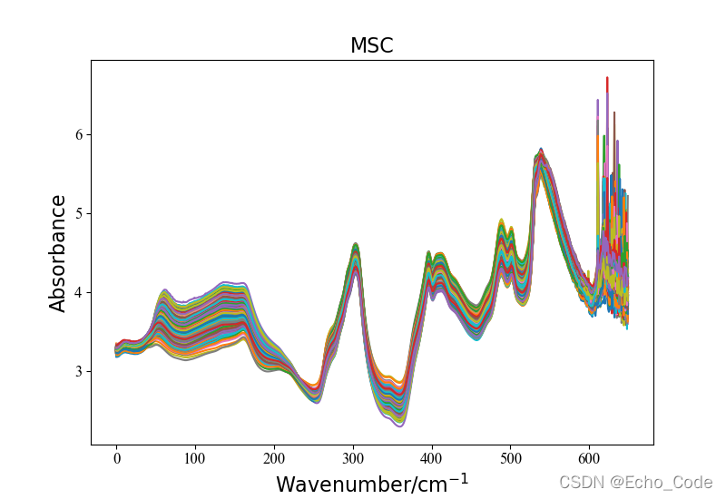
2 .2 光谱预处理的使用

在example.py文件中，提供了光谱预处理模块的使用方法，具体如下，仅需要两行代码即可实现所有常见的光谱预处理。示意1：利用OpenSA实现MSC多元散射校正

 #载入原始数据并可视化
    data, label = LoadNirtest('Rgs')
    plotspc(data, "raw specturm")
    #光谱预处理并可视化
    method = "MSC"
    Preprocessingdata = Preprocessing(method, data)
    plotspc(Preprocessingdata, method)

预处理后的光谱数据如图所示:

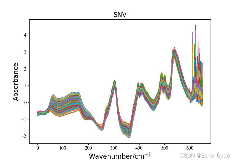
示意2：利用OpenSA实现SNV预处理

    #载入原始数据并可视化
    data, label = LoadNirtest('Rgs')
    plotspc(data, "raw specturm")
    #光谱预处理并可视化
    method = "SNV"
    Preprocessingdata = Preprocessing(method, data)
    plotspc(Preprocessingdata, method)

预处理后的光谱数据如图所示:

总结

利用OpenSA可以非常简单的实现对光谱的预处理，完整代码可从获得GitHub仓库如果对您有用，请点赞！代码现仅供学术使用，若对您的学术研究有帮助，请引用本人的论文，同时，未经许可不得用于商业化应用，欢迎大家继续补充OpenSA中所涉及到的算法，如有问题，微信：Fu_siry

Aiming at the common training datsets split, spectrum preprocessing, wavelength select and calibration models algorithm involved in the spectral analysis process

Related tags

Overview

OpenSA

系列文章目录

前言

一、光谱数据读入

1.1 光谱数据读入

1.2 光谱可视化

二、光谱预处理

2.1 光谱预处理模块

2 .2 光谱预处理的使用

总结

Owner

Fu Pengyou

GND-Nets (Graph Neural Diffusion Networks) in TensorFlow.

Mixed Transformer UNet for Medical Image Segmentation

Tacotron 2 - PyTorch implementation with faster-than-realtime inference

This is the source code of the solver used to compete in the International Timetabling Competition 2019.

Koopman operator identification library in Python

A solution to the 2D Ising model of ferromagnetism, implemented using the Metropolis algorithm

Official repository for the paper F, B, Alpha Matting

ZEBRA: Zero Evidence Biometric Recognition Assessment

Deep Residual Networks with 1K Layers

Demos of essentia classifiers hosted on replicate.ai

Unofficial Implementation of Oboe (SIGCOMM'18').

Official PyTorch implementation of "Meta-Learning with Task-Adaptive Loss Function for Few-Shot Learning" (ICCV2021 Oral)

Training Confidence-Calibrated Classifier for Detecting Out-of-Distribution Samples / ICLR 2018

Python wrapper to access the amazon selling partner API

Detectorch - detectron for PyTorch

Code for ICCV 2021 paper "Distilling Holistic Knowledge with Graph Neural Networks"

An off-line judger supporting distributed problem repositories

rliable is an open-source Python library for reliable evaluation, even with a handful of runs, on reinforcement learning and machine learnings benchmarks.

Unofficial implementation of MLP-Mixer: An all-MLP Architecture for Vision

Codebase for Amodal Segmentation through Out-of-Task andOut-of-Distribution Generalization with a Bayesian Model