House Prices - Advanced Regression Techniques
Predicting House Prices with Machine Learning
This project is build to enhance my knowledge about machine learning and data science project pipeline. If you’re getting into machine learning and want to see a project end to end, please stick around.I will walk you through the steps I’ve taken and attempt to deliver a crash course in machine learning at the same time.
Objective & Data
The Kaggle competition goal is to predict sale prices for homes in Ames, Iowa. You’re given a training and testing data set in csv format as well as a data dictionary.
Training: Our training data consists of 1,460 examples of houses with 79 features describing every aspect of the house. We are given sale prices (labels) for each house. The training data is what we will use to “teach” our models. Testing: The test data set consists of 1,459 examples with the same number of features as the training data. Our test data set excludes the sale price because this is what we are trying to predict. Once our models have been built we will run the best one the test data and submit it to the Kaggle leaderboard.
Task: Machine learning tasks are usually split into three categories; supervised, unsupervised and reinforcement. For this competition, our task is supervised learning.
Tools
I used Python and Jupyter notebooks for the competition. Jupyter notebooks are popular among data scientist because they are easy to follow and show your working steps.
Libraries: These are frameworks in python to handle commonly required tasks. I Implore any budding data scientists to familiarise themselves with these libraries: Pandas — For handling structured data Scikit Learn — For machine learning NumPy — For linear algebra and mathematics Seaborn — For data visualization
Data Cleaning
Kaggle does its best to provide users with clean data. However, we mustn’t become lazy, there are always surprises in the data. Warning! Don’t skip the data cleaning phase, it’s boring but it will save you hours of headache later on.
Duplicates & NaNs: I started by removing duplicates from the data, checked for missing or NaN (not a number) values. It’s important to check for NaNs (and not just because it’s socially moral) because these cause errors in the machine learning models.
Categorical Features: There are a lot of categorical variables that are marked as N/A when a feature of the house is nonexistent. For example, when no alley is present. I identified all the cases where this was happening across the training and test data and replaced the N/As with something more descriptive. N/As can cause errors with machine learning later down the line so get rid of them.
Date Features: For this exercise dates would be better used as categories and not integers. After all, it’s not so much the magnitude that we care about but rather that the dates represent different years. Solving this problem is simple, just convert the numeric dates to strings. Decoded Variables: Some categorical variables had been number encoded. See the example below. 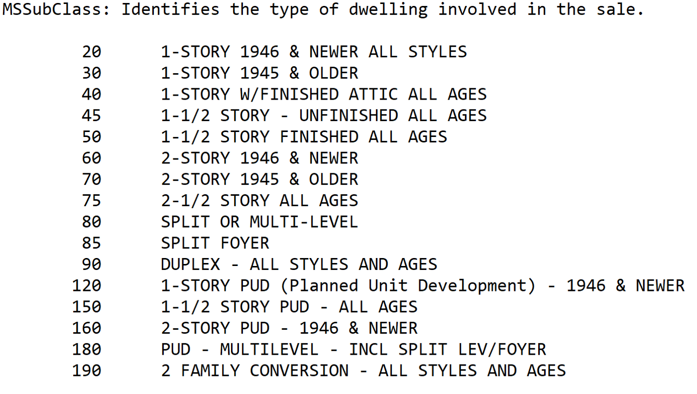
The problem here is that the machine learning algorithm could interpret the magnitude of the number to be important rather than just interpreting it as different categories of a feature. To solve the problem, I reverse engineered the categories and recoded them.
Exploratory Data Analysis (EDA)
This is where our data visualisation journey often begins. The purpose of EDA in machine learning is to explore the quality of our data. A question to keep in mind is; are there any strange patterns that leave us scratching our heads? Labels: I plotted sales price on a histogram. The distribution of sale prices is right skewed, something that is expected. In your neighborhood it might not be unusual to see a few houses that are relatively expensive. Here I perform my first bit of feature engineering (told you the process was messy). I’ll apply a log transform to sales price to compress outliers making the distribution normal. Outliers can have devastating effects on models that use loss functions minimising squared error. Instead of removing outliers try applying a transformation. 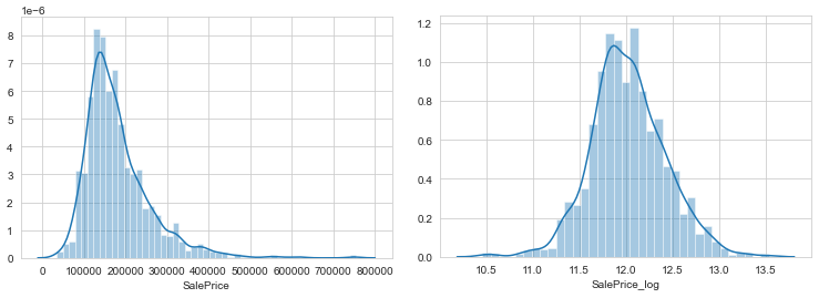
Correlations: It’s often good to plot a correlation matrix to give you an idea of relationships that exist in your data. It can also guide your model building. For example, if you see a lot of your features are correlated with each other you might want to avoid linear regression. 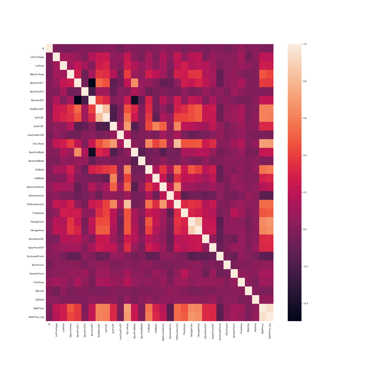 The correlation measure used here is Pearson’s correlation. In our case the lighter the square the stronger the correlation between two variables. Features related to space such as lot frontage, garage area, ground living area were all positively correlated with sale price as one might expect. The logic being that larger properties should be more expensive. No correlations look suspicious here.
Categorical Relations: Sales price appears to be approximately normally distributed within each level of each category. No observations appear, untoward. Some categories contain little to no data, whilst other show little to no distinguishing ability between sales class. See full project on GitHub for data visualisation.
Feature Engineering
Machine learning models can’t understand categorical data. Therefore we will need to apply transformations to convert the categories into numbers. The best practice for doing this is via one hot encoding. OneHotEncoder solves this problem with the options that can be set for categories and handling unknowns. It’s slightly harder to use but definitely necessary for machine learning.
Machine learning
I follow a standard development cycle for machine learning. As a beginner or even a pro, you’ll likely have to go through many iterations of the cycle before you are able to get your models working to a high standard. As you gain more experience the number of iterations will reduce (I promise!).

Model Selection
As mentioned at the start of the article the task is supervised machine learning. We know it’s a regression task because we are being asked to predict a numerical outcome (sale price). Therefore, I approached this problem with three machine learning models. Decision tree, random forest and gradient boosting machines. I used the decision tree as my baseline model then built on this experience to tune my candidate models. This approach saves a lot of time as decision trees are quick to train and can give you an idea of how to tune the hyperparameters for my candidate models.
Training
In machine learning training refers to the process of teaching your model using examples from your training data set. In the training stage, you’ll tune your model hyperparameters.
Hyperparameters: Hyperparameters help us adjust the complexity of our model. There are some best practices on what hyperparameters one should tune for each of the models. I’ll first detail the hyperparameters, then I’ll tell you which I’ve chosen to tune for each model. max_depth — The maximum number of nodes for a given decision tree. max_features — The size of the subset of features to consider for splitting at a node. n_estimators — The number of trees used for boosting or aggregation. This hyperparameter only applies to the random forest and gradient boosting machines. learning_rate — The learning rate acts to reduce the contribution of each tree. This only applies for gradient boosting machines.
Decision Tree — Hyperparameters tuned are the max_depth and the max_features Random Forest — The most important hyperparameters to tune are n_estimators and max_features [1]. Gradient boosting machines — The most important hyperparameters to tune are n_estimators, max_depth and learning_rate [1].
Grid search: Choosing the range of your hyperparameters is an iterative process. With more experience you’ll begin to get a feel for what ranges to set. The good news is once you’ve chosen your possible hyperparameter ranges, grid search allows you to test the model at every combination of those ranges. I’ll talk more about this in the next section. Cross validation: Models are trained with a 5-fold cross validation. A technique that takes the entirety of your training data, randomly splits it into train and validation data sets over 5 iterations. You end up with 5 different training and validation data sets to build and test your models. It’s a good way to counter overfitting.
Implementation
SciKit Learn helps us bring together hyperparameter tuning and cross validation with ease in using GridSearchCv. It gives you options to view the results of each of your training runs.
Evaluation
This is the last step in the process. Here’s where we either jump with joy or pull our hair with frustration (just kidding, we don’t do that…ever). We can use data visualisation to see the results of each of our candidate models. If we are not happy with our results, we might have to revisit our process at any of the stages from data cleaning to machine learning. Our performance metric will be the negative root mean squared error (NRMSE). I’ve used this because it’s the closest I can get to Kaggle’s scoring metric in SciKit Learn.
a) Decision tree: Predictably this was our worst performing method. Our best decision tree score -0.205 NRMSE. Tuning the hyperparameters didn’t appear to make much of a difference to the model’s however it trained in under 2 seconds. There is definitely some scope to assess a wider range of hyperparameters. 
b) Random Forest: Our random forest model was a marked improvement on our decision tree with a NRMSE of -0.144. The model took around 75 seconds to train. 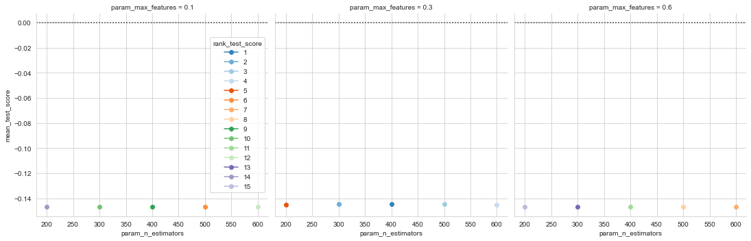
c) Gradient Boosting Machine: This was our best performer by a significant amount with a NRMSE of -0.126. The hyperparameters significantly impact the results illustrating that we must be incredibly careful in how we tune these more complex models. The model took around 196 seconds to train. 
Competition Result
I tested the best performing model on the Kaggle test data. My model put me in the top 39% of entrants (at the time of writing). This isn’t a bad result, but it can definitely be improved.

 32 Apr 24, 2022
 21 Oct 03, 2022
 1 Dec 08, 2021
 575 Jan 01, 2023
 2.2k Jan 08, 2023
 213 Jan 08, 2023
 12 Jan 06, 2023
 1.5k Dec 30, 2022
 7 Oct 11, 2022
 4 Sep 17, 2022
 1 Mar 25, 2022
 105 Dec 28, 2022
 1 Aug 10, 2022
 21 Dec 19, 2022
 91 Dec 02, 2022
 65 Dec 22, 2022
 40 Nov 20, 2022
 19 Oct 27, 2022
 7 Oct 31, 2021
 24 Dec 21, 2022