ThymeBoost
![]()
ThymeBoost combines time series decomposition with gradient boosting to provide a flexible mix-and-match time series framework for spicy forecasting. At the most granular level are the trend/level (going forward this is just referred to as 'trend') models, seasonal models, and endogenous models. These are used to approximate the respective components at each 'boosting round' and sequential rounds are fit on residuals in usual boosting fashion.
Basic flow of the algorithm:

Quick Start.
pip install ThymeBoost
Some basic examples:
Starting with a very simple example of a simple trend + seasonality + noise
import numpy as np
import matplotlib.pyplot as plt
import seaborn as sns
from ThymeBoost import ThymeBoost as tb

sns.set_style('darkgrid')

#Here we will just create a random series with seasonality and a slight trend
seasonality = ((np.cos(np.arange(1, 101))*10 + 50))
np.random.seed(100)
true = np.linspace(-1, 1, 100)
noise = np.random.normal(0, 1, 100)
y = true + noise + seasonality
plt.plot(y)
plt.show()

First we will build the ThymeBoost model object:
boosted_model = tb.ThymeBoost(approximate_splits=True,
                              n_split_proposals=25,
                              verbose=1,
                              cost_penalty=.001)
The arguments passed here are also the defaults. Most importantly, we pass whether we want to use 'approximate splits' and how many splits to propose. If we pass approximate_splits=False then ThymeBoost will exhaustively try every data point to split on if we look for changepoints. If we don't care about changepoints then this is ignored.
ThymeBoost uses a standard fit => predict procedure. Let's use the fit method where everything passed is converted to a itertools cycle object in ThymeBoost, this will be referred as 'generator' parameters moving forward. This might not make sense yet but is shown further in the examples!
output = boosted_model.fit(y,
                           trend_estimator='linear',
                           seasonal_estimator='fourier',
                           seasonal_period=25,
                           split_cost='mse',
                           global_cost='maicc',
                           fit_type='global')
We pass the input time_series and the parameters used to fit. For ThymeBoost the more specific parameters are the different cost functions controlling for each split and the global cost function which controls how many boosting rounds to do. Additionally, the fit_type='global' designates that we are NOT looking for changepoints and just fits our trend_estimator globally.
With verbose ThymeBoost will print out some relevant information for us.
Now that we have fitted our series we can take a look at our results
boosted_model.plot_results(output)

The fit looks correct enough, but let's take a look at the indiviudal components we fitted.
boosted_model.plot_components(output)

Alright, the decomposition looks reasonable as well but let's complicate the task by now adding a changepoint.
Adding a changepoint
true = np.linspace(1, 50, 100)
noise = np.random.normal(0, 1, 100)
y = np.append(y, true + noise + seasonality)
plt.plot(y)
plt.show()

In order to fit this we will change fit_type='global' to fit_type='local'. Let's see what happens.
boosted_model = tb.ThymeBoost(
                            approximate_splits=True,
                            n_split_proposals=25,
                            verbose=1,
                            cost_penalty=.001,
                            )

output = boosted_model.fit(y,
                           trend_estimator='linear',
                           seasonal_estimator='fourier',
                           seasonal_period=25,
                           split_cost='mse',
                           global_cost='maicc',
                           fit_type='local')
predicted_output = boosted_model.predict(output, 100)
Here we add in the predict method which takes in the fitted results as well as the forecast horizon. You will notice that the print out now states we are fitting locally and we do an additional round of boosting. Let's plot the results and see if the new round was ThymeBoost picking up the changepoint.
boosted_model.plot_results(output, predicted_output)

Ok, cool. Looks like it worked about as expected here, we did do 1 wasted round where ThymeBoost just did a slight adjustment at split 80 but that can be fixed as you will see!
Once again looking at the components:
boosted_model.plot_components(output)

There is a kink in the trend right around 100 as to be expected.
Let's further complicate this series.
Adding a large jump
#Pretty complicated model
true = np.linspace(1, 20, 100) + 100
noise = np.random.normal(0, 1, 100)
y = np.append(y, true + noise + seasonality)
plt.plot(y)
plt.show()

So here we have 3 distinct trend lines and one large shift upward. Overall, pretty nasty and automatically fitting this with any model (including ThymeBoost) can have extremely wonky results.
But...let's try anyway. Here we will utilize the 'generator' variables. As mentioned before, everything passed in to the fit method is a generator variable. This basically means that we can pass a list for a parameter and that list will be cycled through at each boosting round. So if we pass this: trend_estimator=['mean', 'linear'] after the initial trend estimation using the median we then use mean followed by linear then mean and linear until boosting is terminated. We can also use this to approximate a potential complex seasonality just by passing a list of what the complex seasonality can be. Let's fit with these generator variables and pay close attention to the print out as it will show you what ThymeBoost is doing at each round.
boosted_model = tb.ThymeBoost(
                            approximate_splits=True,
                            verbose=1,
                            cost_penalty=.001,
                            )

output = boosted_model.fit(y,
                           trend_estimator=['mean'] + ['linear']*20,
                           seasonal_estimator='fourier',
                           seasonal_period=[25, 0],
                           split_cost='mae',
                           global_cost='maicc',
                           fit_type='local',
                           connectivity_constraint=True,
                           )

predicted_output = boosted_model.predict(output, 100)
The log tells us what we need to know:
********** Round 1 **********
Using Split: None
Fitting initial trend globally with trend model:
median()
seasonal model:
fourier(10, False)
cost: 2406.7734967780552
********** Round 2 **********
Using Split: 200
Fitting local with trend model:
mean()
seasonal model:
None
cost: 1613.03414289753
********** Round 3 **********
Using Split: 174
Fitting local with trend model:
linear((1, None))
seasonal model:
fourier(10, False)
cost: 1392.923553270366
********** Round 4 **********
Using Split: 274
Fitting local with trend model:
linear((1, None))
seasonal model:
None
cost: 1384.306737800115
==============================
Boosting Terminated
Using round 4
The initial round for trend is always the same (this idea is pretty core to the boosting framework) but after that we fit with mean and the next 2 rounds are fit with linear estimation. The complex seasonality works 100% as we expect, just going back and forth between the 2 periods we give it where a 0 period means no seasonality estimation occurs.
Let's take a look at the results:
boosted_model.plot_results(output, predicted_output)

Hmmm, that looks very wonky.
But since we used a mean estimator we are saying that there is a change in the overall level of the series. That's not exactly true, by appending that last series with just another trend line we essentially changed the slope and the intercept of the series.
To account for this, let's relax connectivity constraints and just try linear estimators. Once again, EVERYTHING passed to the fit method is a generator variable so we will relax the connectivity constraint for the first linear fit to hopefully account for the large jump. After that we will use the constraint for 10 rounds then ThymeBoost will just cycle through the list we provide again.
#Without connectivity constraint
boosted_model = tb.ThymeBoost(
approximate_splits=True,
verbose=1,
cost_penalty=.001,
)
output = boosted_model.fit(y,
trend_estimator='linear',
seasonal_estimator='fourier',
seasonal_period=[25, 0],
split_cost='mae',
global_cost='maicc',
fit_type='local',
connectivity_constraint=[False] + [True]*10,
)
predicted_output = boosted_model.predict(output, 100)
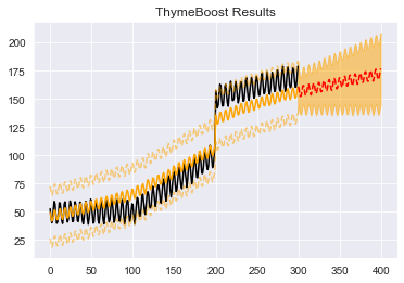
boosted_model.plot_results(output, predicted_output)

Alright, that looks a ton better. It does have some underfitting going on in the middle which is typical since we are using binary segmentation for the changepoints. But other than that it seems reasonable. Let's take a look at the components:
boosted_model.plot_components(output)

Looks like the model is catching on to the underlying process creating the data. The trend is clearly composed of three segments and has that large jump right at 200 just as we hoped to see!
Controlling the boosting rounds
We can control how many rounds and therefore the complexity of our model a couple of different ways. The most direct is by controlling the number of rounds.
#n_rounds=1
boosted_model = tb.ThymeBoost(
                            approximate_splits=True,
                            verbose=1,
                            cost_penalty=.001,
                            n_rounds=1
                            )

output = boosted_model.fit(y,
                           trend_estimator='arima',
                           arima_order=[(1, 0, 0), (1, 0, 1), (1, 1, 1)],
                           seasonal_estimator='fourier',
                           seasonal_period=25,
                           split_cost='mae',
                           global_cost='maicc',
                           fit_type='global',
                           )
predicted_output = boosted_model.predict(output, 100)
boosted_model.plot_components(output)

By passing n_rounds=1 we only allow ThymeBoost to do the initial trend estimation (a simple median) and one shot at approximating the seasonality.
Additionally we are trying out a new trend_estimator along with the related parameter arima_order. Although we didn't get to it we are passing the arima_order to go from simple to complex.
Let's try forcing ThymeBoost to go through all of our provided ARIMA orders by setting n_rounds=4
boosted_model = tb.ThymeBoost(
                            approximate_splits=True,
                            verbose=1,
                            cost_penalty=.001,
                            n_rounds=4,
                            regularization=1.2
                            )

output = boosted_model.fit(y,
                           trend_estimator='arima',
                           arima_order=[(1, 0, 0), (1, 0, 1), (1, 1, 1)],
                           seasonal_estimator='fourier',
                           seasonal_period=25,
                           split_cost='mae',
                           global_cost='maicc',
                           fit_type='global',
                           )
predicted_output = boosted_model.predict(output, 100)
Looking at the log:
********** Round 1 **********
Using Split: None
Fitting initial trend globally with trend model:
median()
seasonal model:
fourier(10, False)
cost: 2406.7734967780552
********** Round 2 **********
Using Split: None
Fitting global with trend model:
arima((1, 0, 0))
seasonal model:
fourier(10, False)
cost: 988.0694403606061
********** Round 3 **********
Using Split: None
Fitting global with trend model:
arima((1, 0, 1))
seasonal model:
fourier(10, False)
cost: 991.7292716360867
********** Round 4 **********
Using Split: None
Fitting global with trend model:
arima((1, 1, 1))
seasonal model:
fourier(10, False)
cost: 1180.688829140743
We can see that the cost which typically controls boosting is ignored. It actually increases in round 3. An alternative for boosting complexity would be to pass a larger regularization parameter when building the model class.
Component Regularization with a Learning Rate
Another idea taken from gradient boosting is the use of a learning rate. However, we allow component-specific learning rates. The main benefit to this is that it allows us to have the same fitting procedure (always trend => seasonality => exogenous) but account for the potential different ways we want to fit. For example, let's say our series is responding to an exogenous variable that is seasonal. Since we fit for seasonality BEFORE exogenous then we could eat up that signal. However, we could simply pass a seasonality_lr (or trend_lr / exogenous_lr) which will penalize the seasonality approximation and leave the signal for the exogenous component fit.
Here is a quick example, as always we could pass it as a list if we want to allow seasonality to return to normal after the first round.
#seasonality regularization
boosted_model = tb.ThymeBoost(
                            approximate_splits=True,
                            verbose=1,
                            cost_penalty=.001,
                            n_rounds=2
                            )

output = boosted_model.fit(y,
                           trend_estimator='arima',
                           arima_order=(1, 0, 1),
                           seasonal_estimator='fourier',
                           seasonal_period=25,
                           split_cost='mae',
                           global_cost='maicc',
                           fit_type='global',
                           seasonality_lr=.1
                           )
predicted_output = boosted_model.predict(output, 100)
Parameter Optimization
ThymeBoost has an optimizer which will try to find the 'optimal' parameter settings based on all combinations that are passed.
Importantly, all parameters that are normally pass to fit must now be passed as a list.
Let's take a look:
boosted_model = tb.ThymeBoost(
                           approximate_splits=True,
                           verbose=0,
                           cost_penalty=.001,
                           )

output = boosted_model.optimize(y,
                                verbose=1,
                                lag=20,
                                optimization_steps=1,
                                trend_estimator=['mean', 'linear', ['mean', 'linear']],
                                seasonal_period=[0, 25],
                                fit_type=['local', 'global'])
100%|██████████| 12/12 [00:00<00:00, 46.63it/s]
Optimal model configuration: {'trend_estimator': 'linear', 'fit_type': 'local', 'seasonal_period': 25, 'exogenous': None}
Params ensembled: False
First off, I disabled the verbose call in the constructor so it won't print out everything for each model. Instead, passing verbose=1 to the optimize method will print a tqdm progress bar and the best model configuration. Lag refers to the number of points to holdout for our test set and optimization_steps allows you to roll through the holdout.
Another important thing to note, one of the elements in the list of trend_estimators is itself a list. With optimization, all we do is try each combination of the parameters given so each element in the list provided will be passed to the normal fit method, if that element is a list then that means you are using a generator variable for that implementation.
With the optimizer class we retain all other methods we have been using after fit.
predicted_output = boosted_model.predict(output, 100)

boosted_model.plot_results(output, predicted_output)

So this output looks wonky around that changepoint but it recovers in time to produce a good enough forecast to do well in the holdout.
Ensembling
Instead of iterating through and choosing the best parameters we could also just ensemble them into a simple average of every parameter setting.
Everything stated about the optimizer holds for ensemble as well, except now we just call the ensemble method.
boosted_model = tb.ThymeBoost(
                           approximate_splits=True,
                           verbose=0,
                           cost_penalty=.001,
                           )

output = boosted_model.ensemble(y,
                                trend_estimator=['mean', 'linear', ['mean', 'linear']],
                                seasonal_period=[0, 25],
                                fit_type=['local', 'global'])

predicted_output = boosted_model.predict(output, 100)

boosted_model.plot_results(output, predicted_output)
Obviously, this output is quite wonky. Primarily because of the 'global' parameter which is pulling everything to the center of the data. However, ensembling has been shown to be quite effective in the wild.
Optimization with Ensembling?
So what if we want to try an ensemble out during optimization, is that possible?
The answer is yes!
But to do it we have to use a new function in our optimize method. Here is an example:
boosted_model = tb.ThymeBoost(
                           approximate_splits=True,
                           verbose=0,
                           cost_penalty=.001,
                           )

output = boosted_model.optimize(y,
                                lag=10,
                                optimization_steps=1,
                                trend_estimator=['mean', boosted_model.combine(['ses', 'des', 'damped_des'])],
                                seasonal_period=[0, 25],
                                fit_type=['global'])

predicted_output = boosted_model.predict(output, 100)
For everything we want to be treated as an ensemble while optimizing we must wrap the parameter list in the combine function as seen: boosted_model.combine(['ses', 'des', 'damped_des'])
And now in the log:
Optimal model configuration: {'trend_estimator': ['ses', 'des', 'damped_des'], 'fit_type': ['global'], 'seasonal_period': [25], 'exogenous': [None]}
Params ensembled: True
We see that everything returned is a list and 'Params ensembled' is now True, signifying to ThymeBoost that this is an Ensemble.
Let's take a look at the outputs:
boosted_model.plot_results(output, predicted_output)

ToDo
The package is still under heavy development and with the large number of combinations that arise from the framework if you find any issues definitely raise them!
Logging and error handling is still basic to non-existent, so it is one of our top priorities.

 1 Dec 17, 2021
 5.6k Dec 30, 2022
 35 Nov 06, 2022
 217 Dec 12, 2022
 4 Jul 25, 2022
 84 Dec 26, 2022
 427 Dec 27, 2022
 1 Dec 02, 2021
 33k Dec 28, 2022
 12 May 30, 2022
 1 Nov 16, 2022
 40 Sep 19, 2022
 16 Dec 15, 2022
 3 May 03, 2022
 1 Jan 12, 2022
 23 Dec 20, 2022
 29 May 22, 2022
 7 Aug 23, 2022
 3 Apr 20, 2022
 4 Sep 13, 2022