数据挖掘流程：

（一）数据读取：

• 读取数据，并进行展示

• 统计数据各项指标

• 明确数据规模与要完成任务
  （二）特征理解分析

• 单特征分析，逐个变量分析其对结果的影响

• 多变量统计分析，综合考虑多种情况影响

• 统计绘图得出结论
  （三）数据清洗与预处理

• 对缺失值进行填充

• 特征标准化/归一化

• 筛选有价值的特征

• 分析特征之间的相关性
  （四）建立模型

• 特征数据与标签准备

• 数据集切分

• 多种建模算法对比

• 集成策略等方案改进

import numpy as np 
import pandas as pd
import matplotlib.pyplot as plt
import seaborn as sns
plt.style.use('fivethirtyeight')
import warnings
warnings.filterwarnings('ignore')
%matplotlib inline

数据读取

data=pd.read_csv('train.csv')
data.head()

查看有没有缺失值

data.isnull().sum() #checking for total null values

整体看看数据啥规模

data.describe()

不是要预测这大船的获救情况嘛，先看看获救比例咋样

f,ax=plt.subplots(1,2,figsize=(18,8))
data['Survived'].value_counts().plot.pie(explode=[0,0.1],autopct='%1.1f%%',ax=ax[0],shadow=True)
ax[0].set_title('Survived')
ax[0].set_ylabel('')
sns.countplot('Survived',data=data,ax=ax[1])
ax[1].set_title('Survived')
plt.show()

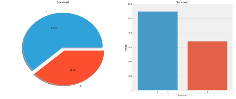显然，这次事故中没有多少乘客幸免于难。

在训练集的891名乘客中，只有大约350人幸存下来，只有38.4%的机组人员在空难中幸存下来。我们需要从数据中挖掘出更多的信息，看看哪些类别的乘客幸存下来，哪些没有。

我们将尝试使用数据集的不同特性来检查生存率。比如性别，年龄，登船地点等，但是首先我们得来理解下数据中的特征！

数据特征分为：连续值和离散值

• 离散值：性别（男，女） 登船地点（S,Q,C）
• 连续值：年龄，船票价格

data.groupby(['Sex','Survived'])['Survived'].count()

f,ax=plt.subplots(1,2,figsize=(18,8))
data[['Sex','Survived']].groupby(['Sex']).mean().plot.bar(ax=ax[0])
ax[0].set_title('Survived vs Sex')
sns.countplot('Sex',hue='Survived',data=data,ax=ax[1])
ax[1].set_title('Sex:Survived vs Dead')
plt.show()

这看起来很有趣。船上的男人比女人多得多。不过，挽救的女性人数几乎是男性的两倍。生存率为一个女人在船上是75%左右，而男性在18-19%左右。（让妇女和儿童先走，虽然电影忘得差不多了，这句话还记着。。。确实是这样的）

Pclass --> 船舱等级跟获救情况的关系

pd.crosstab(data.Pclass,data.Survived,margins=True).style.background_gradient(cmap='summer_r')#交叉表

f,ax=plt.subplots(1,2,figsize=(18,8))
data['Pclass'].value_counts().plot.bar(color=['#CD7F32','#FFDF00','#D3D3D3'],ax=ax[0])
ax[0].set_title('Number Of Passengers By Pclass')
ax[0].set_ylabel('Count')
sns.countplot('Pclass',hue='Survived',data=data,ax=ax[1])
ax[1].set_title('Pclass:Survived vs Dead')
plt.show()

人们说金钱不能买到一切。但我们可以清楚地看到，船舱等级为1的被给予很高的优先级而救援。尽管数量在pClass 3乘客高了很多，仍然存活数从他们是非常低的，大约25%。

对于pClass1来说存活是63%左右，而pclass2大约是48%。所以金钱和地位很重要。这样一个物欲横流的世界。

那这些又和性别有关吗？接下来我们再来看看船舱等级和性别对结果的影响

pd.crosstab([data.Sex,data.Survived],data.Pclass,margins=True).style.background_gradient(cmap='summer_r')

sns.factorplot('Pclass','Survived',hue='Sex',data=data)
plt.show()

我们用factorplot这个图，看起来更直观一些。

我们可以很容易地推断，从pclass1女性生存是95-96%，如94人中只有3的女性从pclass1没获救。

显而易见的是，不论pClass，女性优先考虑。

看来Pclass也是一个重要的特征。让我们分析其他特征

Age–> 连续值特征对结果的影响

f,ax=plt.subplots(1,2,figsize=(18,8))
sns.violinplot("Pclass","Age", hue="Survived", data=data,split=True,ax=ax[0])
ax[0].set_title('Pclass and Age vs Survived')
ax[0].set_yticks(range(0,110,10))
sns.violinplot("Sex","Age", hue="Survived", data=data,split=True,ax=ax[1])
ax[1].set_title('Sex and Age vs Survived')
ax[1].set_yticks(range(0,110,10))
plt.show()

结果：¶ 1）10岁以下儿童的存活率随passenegers数量增加。

2）生存为20-50岁获救几率更高一些。

3）对男性来说，随着年龄的增长，存活率降低。

缺失值填充

• 平均值
• 经验值
• 回归模型预测
• 剔除掉

正如我们前面看到的，年龄特征有177个空值。为了替换这些缺失值，我们可以给它们分配数据集的平均年龄。

但问题是，有许多不同年龄的人。最好的办法是找到一个合适的年龄段！

我们可以检查名字特征。根据这个特征，我们可以看到名字有像先生或夫人这样的称呼，这样我们就可以把先生和夫人的平均值分配给各自的组。

data['Initial']=0
for i in data:
    data['Initial']=data.Name.str.extract('([A-Za-z]+)\.') 

好了，这里我们使用正则表达式：[A-Za-z] +）来提取信息

pd.crosstab(data.Initial,data.Sex).T.style.background_gradient(cmap='summer_r') 

data['Initial'].replace(['Mlle','Mme','Ms','Dr','Major','Lady','Countess','Jonkheer','Col','Rev','Capt','Sir','Don'],['Miss','Miss','Miss','Mr','Mr','Mrs','Mrs','Other','Other','Other','Mr','Mr','Mr'],inplace=True)

data.groupby('Initial')['Age'].mean() 

填充缺失值

## 使用每组的均值来进行填充
data.loc[(data.Age.isnull())&(data.Initial=='Mr'),'Age']=33
data.loc[(data.Age.isnull())&(data.Initial=='Mrs'),'Age']=36
data.loc[(data.Age.isnull())&(data.Initial=='Master'),'Age']=5
data.loc[(data.Age.isnull())&(data.Initial=='Miss'),'Age']=22
data.loc[(data.Age.isnull())&(data.Initial=='Other'),'Age']=46

f,ax=plt.subplots(1,2,figsize=(20,10))
data[data['Survived']==0].Age.plot.hist(ax=ax[0],bins=20,edgecolor='black',color='red')
ax[0].set_title('Survived= 0')
x1=list(range(0,85,5))
ax[0].set_xticks(x1)
data[data['Survived']==1].Age.plot.hist(ax=ax[1],color='green',bins=20,edgecolor='black')
ax[1].set_title('Survived= 1')
x2=list(range(0,85,5))
ax[1].set_xticks(x2)
plt.show()

观察:

1）幼儿（年龄在5岁以下）获救的还是蛮多的（妇女和儿童优先政策）。

2）最老的乘客得救了（80年）。

3）死亡人数最高的是30-40岁年龄组。

sns.factorplot('Pclass','Survived',col='Initial',data=data)
plt.show()

特征之间的相关性

sns.heatmap(data.corr(),annot=True,cmap='RdYlGn',linewidths=0.2) #data.corr()-->correlation matrix
fig=plt.gcf()
fig.set_size_inches(10,8)
plt.show()

特征相关性的热度图

首先要注意的是，只有数值特征进行比较

正相关：如果特征A的增加导致特征b的增加，那么它们呈正相关。值1表示完全正相关。

负相关：如果特征A的增加导致特征b的减少，则呈负相关。值-1表示完全负相关。

现在让我们说两个特性是高度或完全相关的，所以一个增加导致另一个增加。这意味着两个特征都包含高度相似的信息，并且信息很少或没有变化。这样的特征对我们来说是没有价值的！

那么你认为我们应该同时使用它们吗？。在制作或训练模型时，我们应该尽量减少冗余特性，因为它减少了训练时间和许多优点。

现在，从上面的图，我们可以看到，特征不显著相关。

特征工程和数据清洗

当我们得到一个具有特征的数据集时，是不是所有的特性都很重要？可能有许多冗余的特征应该被消除，我们还可以通过观察或从其他特征中提取信息来获得或添加新特性。

年龄特征：

正如我前面提到的，年龄是连续的特征，在机器学习模型中存在连续变量的问题。

如果我说通过性别来组织或安排体育运动，我们可以很容易地把他们分成男女分开。

如果我说按他们的年龄分组，你会怎么做？如果有30个人，可能有30个年龄值。

我们需要对连续值进行离散化来分组。

好的，乘客的最大年龄是80岁。所以我们将范围从0-80成5箱。所以80/5＝16。

data['Age_band']=0
data.loc[data['Age']<=16,'Age_band']=0
data.loc[(data['Age']>16)&(data['Age']<=32),'Age_band']=1
data.loc[(data['Age']>32)&(data['Age']<=48),'Age_band']=2
data.loc[(data['Age']>48)&(data['Age']<=64),'Age_band']=3
data.loc[data['Age']>64,'Age_band']=4
data.head(2)

data['Age_band'].value_counts().to_frame().style.background_gradient(cmap='summer')

sns.factorplot('Age_band','Survived',data=data,col='Pclass')
plt.show()

生存率随年龄的增加而减少，不论Pclass。

Family_size：家庭总人数

data['Family_Size']=0
data['Family_Size']=data['Parch']+data['SibSp']#family size
data['Alone']=0
data.loc[data.Family_Size==0,'Alone']=1#Alone

f,ax=plt.subplots(1,2,figsize=(18,6))
sns.factorplot('Family_Size','Survived',data=data,ax=ax[0])
ax[0].set_title('Family_Size vs Survived')
sns.factorplot('Alone','Survived',data=data,ax=ax[1])
ax[1].set_title('Alone vs Survived')
plt.close(2)
plt.close(3)
plt.show()

family_size = 0意味着passeneger是孤独的。显然，如果你是单独或family_size = 0，那么生存的机会很低。家庭规模4以上，机会也减少。这看起来也是模型的一个重要特性。

将字符串值转换为数字 因为我们不能把字符串一个机器学习模型

data['Sex'].replace(['male','female'],[0,1],inplace=True)
data['Embarked'].replace(['S','C','Q'],[0,1,2],inplace=True)
data['Initial'].replace(['Mr','Mrs','Miss','Master','Other'],[0,1,2,3,4],inplace=True)

去掉不必要的特征

名称>我们不需要name特性，因为它不能转换成任何分类值

年龄——>我们有age_band特征，所以不需要这个

票号–>这是任意的字符串，不能被归类

票价——>我们有fare_cat特征，所以不需要

船仓号——>这个也不要没啥含义

passengerid -->不能被归类

data.drop(['Name','Age','Ticket','Fare','Cabin','Fare_Range','PassengerId'],axis=1,inplace=True)
sns.heatmap(data.corr(),annot=True,cmap='RdYlGn',linewidths=0.2,annot_kws={
    'size':20})
fig=plt.gcf()
fig.set_size_inches(18,15)
plt.xticks(fontsize=14)
plt.yticks(fontsize=14)
plt.show()

现在以上的相关图，我们可以看到一些正相关的特征。他们中的一些人sibsp和family_size和干燥family_size和一些负面的孤独和family_size。

机器学习建模

现在我们将使用一些很好的分类算法来预测乘客是否能生存下来：

1）logistic回归

2）支持向量机（线性和径向）

3）随机森林

4）k-近邻

5）朴素贝叶斯

6）决策树

7）神经网络

from sklearn.linear_model import LogisticRegression 
from sklearn import svm 
from sklearn.ensemble import RandomForestClassifier
from sklearn.neighbors import KNeighborsClassifier
from sklearn.naive_bayes import GaussianNB 
from sklearn.tree import DecisionTreeClassifier
from sklearn.model_selection import train_test_split
from sklearn import metrics 
from sklearn.metrics import confusion_matrix 

train,test=train_test_split(data,test_size=0.3,random_state=0,stratify=data['Survived'])
train_X=train[train.columns[1:]]
train_Y=train[train.columns[:1]]
test_X=test[test.columns[1:]]
test_Y=test[test.columns[:1]]
X=data[data.columns[1:]]
Y=data['Survived']

SVM

model=svm.SVC(kernel='rbf',C=1,gamma=0.1)
model.fit(train_X,train_Y)
prediction1=model.predict(test_X)
print('Accuracy for rbf SVM is ',metrics.accuracy_score(prediction1,test_Y))

linear-SVM

model=svm.SVC(kernel='linear',C=0.1,gamma=0.1)
model.fit(train_X,train_Y)
prediction2=model.predict(test_X)
print('Accuracy for linear SVM is',metrics.accuracy_score(prediction2,test_Y))

Logistic Regression

model = LogisticRegression()
model.fit(train_X,train_Y)
prediction3=model.predict(test_X)
print('The accuracy of the Logistic Regression is',metrics.accuracy_score(prediction3,test_Y))

Decision Tree

model=DecisionTreeClassifier()
model.fit(train_X,train_Y)
prediction4=model.predict(test_X)
print('The accuracy of the Decision Tree is',metrics.accuracy_score(prediction4,test_Y))

KNN

model=KNeighborsClassifier() 
model.fit(train_X,train_Y)
prediction5=model.predict(test_X)
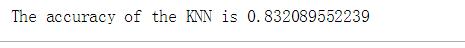
print('The accuracy of the KNN is',metrics.accuracy_score(prediction5,test_Y))

现在的精度为KNN模型的变化，我们改变n_neighbours值属性。默认值是5。让我们检查的精度在n_neighbours不同时的结果。

a_index=list(range(1,11))
a=pd.Series()
x=[0,1,2,3,4,5,6,7,8,9,10]
for i in list(range(1,11)):
    model=KNeighborsClassifier(n_neighbors=i) 
    model.fit(train_X,train_Y)
    prediction=model.predict(test_X)
    a=a.append(pd.Series(metrics.accuracy_score(prediction,test_Y)))
plt.plot(a_index, a)
plt.xticks(x)
fig=plt.gcf()
fig.set_size_inches(12,6)
plt.show()
print('Accuracies for different values of n are:',a.values,'with the max value as ',a.values.max())

model=GaussianNB()
model.fit(train_X,train_Y)
prediction6=model.predict(test_X)
print('The accuracy of the NaiveBayes is',metrics.accuracy_score(prediction6,test_Y))

模型的精度并不是决定分类器效果的唯一因素。假设分类器在训练数据上进行训练，需要在测试集上进行测试才有效果

现在这个分类器的精确度很高，但是我们可以确认所有的新测试集都是90%吗？答案是否定的，因为我们不能确定分类器在不同数据源上的结果。当训练和测试数据发生变化时，精确度也会改变。它可能会增加或减少。

为了克服这一点，得到一个广义模型，我们使用交叉验证。

交叉验证！

一个测试集看起来不太够呀，多轮求均值是一个好的策略！

1）的交叉验证的工作原理是首先将数据集分成k-subsets。

2）假设我们将数据集划分为（k＝5）部分。我们预留1个部分进行测试，并对这4个部分进行训练。

3）我们通过在每次迭代中改变测试部分并在其他部分中训练算法来继续这个过程。然后对衡量结果求平均值，得到算法的平均精度。

这就是所谓的交叉验证。

from sklearn.model_selection import KFold #for K-fold cross validation
from sklearn.model_selection import cross_val_score #score evaluation
from sklearn.model_selection import cross_val_predict #prediction
kfold = KFold(n_splits=10, random_state=22) # k=10, split the data into 10 equal parts
xyz=[]
accuracy=[]
std=[]
classifiers=['Linear Svm','Radial Svm','Logistic Regression','KNN','Decision Tree','Naive Bayes','Random Forest']
models=[svm.SVC(kernel='linear'),svm.SVC(kernel='rbf'),LogisticRegression(),KNeighborsClassifier(n_neighbors=9),DecisionTreeClassifier(),GaussianNB(),RandomForestClassifier(n_estimators=100)]
for i in models:
    model = i
    cv_result = cross_val_score(model,X,Y, cv = kfold,scoring = "accuracy")
    cv_result=cv_result
    xyz.append(cv_result.mean())
    std.append(cv_result.std())
    accuracy.append(cv_result)
new_models_dataframe2=pd.DataFrame({
    'CV Mean':xyz,'Std':std},index=classifiers)       
new_models_dataframe2

plt.subplots(figsize=(12,6))
box=pd.DataFrame(accuracy,index=[classifiers])
box.T.boxplot()

new_models_dataframe2['CV Mean'].plot.barh(width=0.8)
plt.title('Average CV Mean Accuracy')
fig=plt.gcf()
fig.set_size_inches(8,5)
plt.show()

f,ax=plt.subplots(3,3,figsize=(12,10))
y_pred = cross_val_predict(svm.SVC(kernel='rbf'),X,Y,cv=10)
sns.heatmap(confusion_matrix(Y,y_pred),ax=ax[0,0],annot=True,fmt='2.0f')
ax[0,0].set_title('Matrix for rbf-SVM')
y_pred = cross_val_predict(svm.SVC(kernel='linear'),X,Y,cv=10)
sns.heatmap(confusion_matrix(Y,y_pred),ax=ax[0,1],annot=True,fmt='2.0f')
ax[0,1].set_title('Matrix for Linear-SVM')
y_pred = cross_val_predict(KNeighborsClassifier(n_neighbors=9),X,Y,cv=10)
sns.heatmap(confusion_matrix(Y,y_pred),ax=ax[0,2],annot=True,fmt='2.0f')
ax[0,2].set_title('Matrix for KNN')
y_pred = cross_val_predict(RandomForestClassifier(n_estimators=100),X,Y,cv=10)
sns.heatmap(confusion_matrix(Y,y_pred),ax=ax[1,0],annot=True,fmt='2.0f')
ax[1,0].set_title('Matrix for Random-Forests')
y_pred = cross_val_predict(LogisticRegression(),X,Y,cv=10)
sns.heatmap(confusion_matrix(Y,y_pred),ax=ax[1,1],annot=True,fmt='2.0f')
ax[1,1].set_title('Matrix for Logistic Regression')
y_pred = cross_val_predict(DecisionTreeClassifier(),X,Y,cv=10)
sns.heatmap(confusion_matrix(Y,y_pred),ax=ax[1,2],annot=True,fmt='2.0f')
ax[1,2].set_title('Matrix for Decision Tree')
y_pred = cross_val_predict(GaussianNB(),X,Y,cv=10)
sns.heatmap(confusion_matrix(Y,y_pred),ax=ax[2,0],annot=True,fmt='2.0f')
ax[2,0].set_title('Matrix for Naive Bayes')
plt.subplots_adjust(hspace=0.2,wspace=0.2)
plt.show()

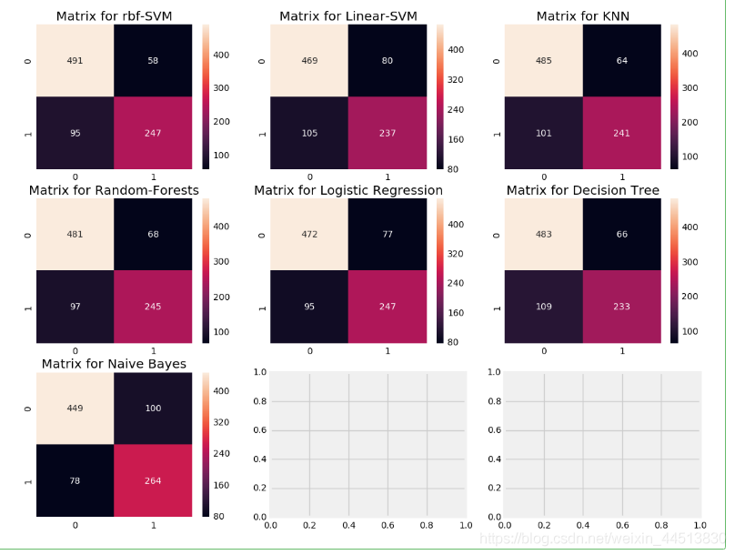解释混淆矩阵：来看第一个图

1）预测的正确率为491（死亡）+ 247（存活），平均CV准确率为（491+247）/ 891＝82.8%。

2）58和95都是咱们弄错了的。

超参数整定

机器学习模型就像一个黑盒子。这个黑盒有一些默认参数值，我们可以调整或更改以获得更好的模型。比如支持向量机模型中的C和γ，我们称之为超参数，他们对结果可能产生非常大的影响。

from sklearn.model_selection import GridSearchCV
C=[0.05,0.1,0.2,0.3,0.25,0.4,0.5,0.6,0.7,0.8,0.9,1]
gamma=[0.1,0.2,0.3,0.4,0.5,0.6,0.7,0.8,0.9,1.0]
kernel=['rbf','linear']
hyper={
    'kernel':kernel,'C':C,'gamma':gamma}
gd=GridSearchCV(estimator=svm.SVC(),param_grid=hyper,verbose=True)
gd.fit(X,Y)
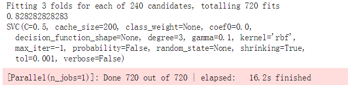
print(gd.best_score_)
print(gd.best_estimator_)

Random Forests

n_estimators=range(100,1000,100)
hyper={
    'n_estimators':n_estimators}
gd=GridSearchCV(estimator=RandomForestClassifier(random_state=0),param_grid=hyper,verbose=True)
gd.fit(X,Y)
print(gd.best_score_)
print(gd.best_estimator_)

RBF支持向量机的最佳得分为82.82%，C＝0.5，γ＝0.1。RandomForest，成绩是81.8%