Tips ： After writing the article , Directories can be generated automatically , How to generate it, please refer to the help document on the right

Preface

This paper is based on 《Pytorch Deep learning practice 》 Study notes sorted out by the contents of Chapter 6 of a book
Explanation of relevant codes and corresponding expansion .

The code used in this article is based on jupyter

1. neural network

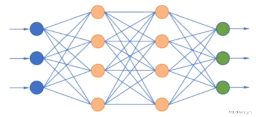
The core of deep learning is neural network ： A mathematical entity that can represent complex functions through the combination of simple functions

The basic building blocks of these complex functions are neurons , Its core is the linear transformation of input and then the application of a fixed nonlinear function , The activation function .

Mathematically , We can write it as o = f(wx+b), among x It's input ,w Is a weight or scale factor ,b Is offset or offset ,f Is the activation function . Usually ,x and o It can be a simple scalar , Or vector value ,w It can be a single scalar or matrix , and b Is scalar or vector . In the latter case , The previous expression is called a layer of neurons .

1.1. Form a multilayer network

1.2. Understand the error function

An important difference between our previous linear model and the model we will actually use for deep learning is the shape of the error function . Our linear model and error squared loss function have a convex error curve , It has a strange 、 Clearly defined minimum . If you use other methods , It can be automatic 、 Determine the parameter that minimizes the value of the error function , This means that our parameter update attempts to estimate the singular correct answer as much as possible .

Even if the same error square loss function is used , Neural networks also do not have the same characteristics as convex error surfaces ！ For every parameter we try to approximate , There is no single correct answer . contrary , We try to make all the parameters , When synergistic , Produce a useful output . Because this useful output is only close to the fact , So there will be a certain degree of imperfection .

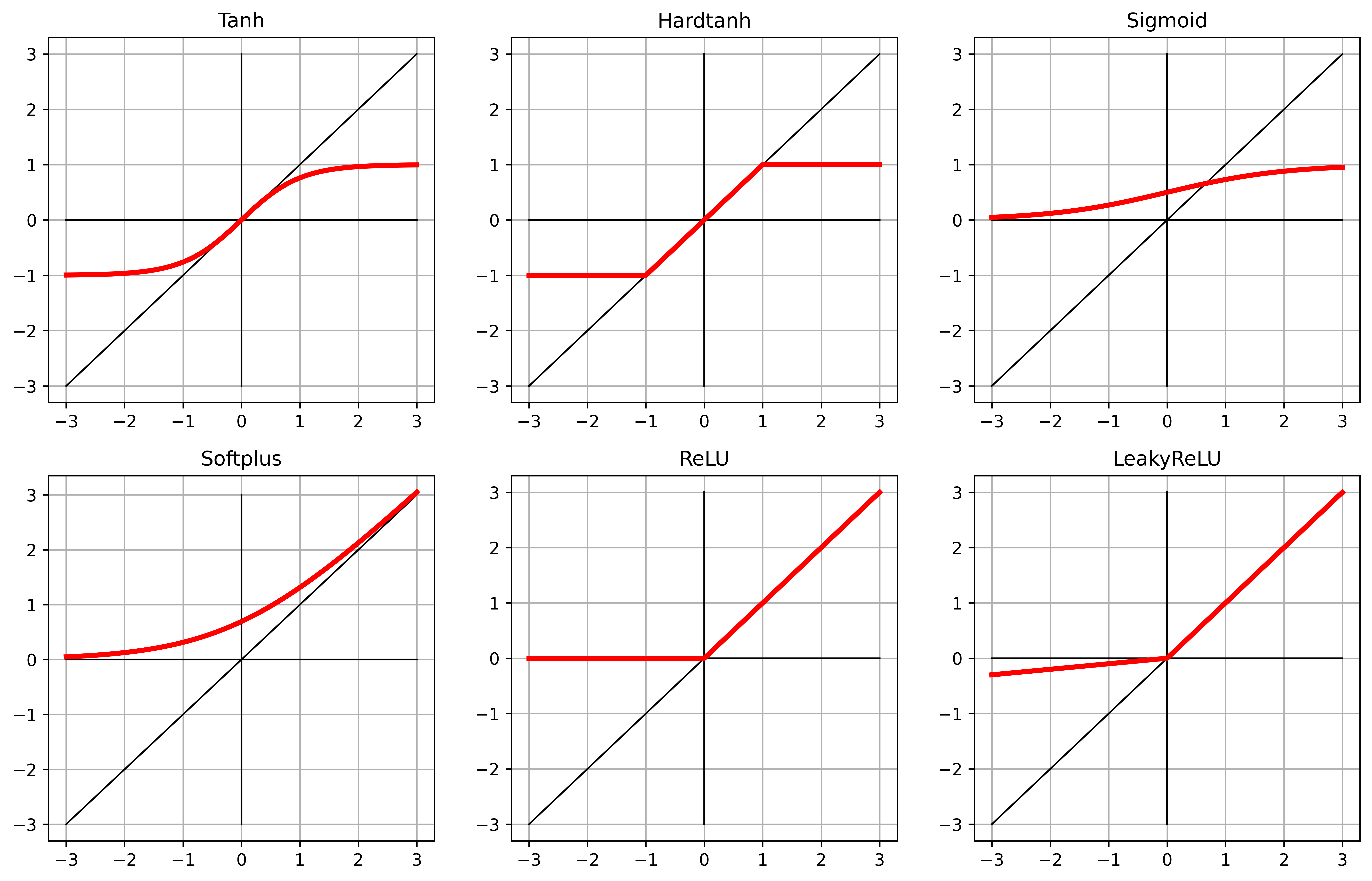
1.3. Activation function

Activate the 2 It's an important role ：

• Inside the model , It allows the output function to have different slopes on different values , This is something linear functions can't do . By cleverly setting different slopes for many outputs , Neural network can approximate any function
• At the last layer of the network , Its function is to concentrate the output of the previous linear operation within a given range
  1. Limit the output range
     Set the output value online
     torch.nn.Hardtanh()
  2. Compress the output range
     torch.nn.Sigmoid()
     The curves of these functions are x As it approaches negative infinity, it gradually approaches 0 or -1, With x To approach gradually 1, Function in x==0 It has a basically constant slope

1.4. Choose the best activation function

The activation function has the following characteristics ：

1. The activation function is nonlinear
2. The activation function is differentiable , So they can calculate the gradient

The reality of the function ：

1. They have at least one sensitive area , In this range , The change of input will lead to the corresponding change of output
2. They contain many insensitivity （ Or saturation ） The scope of the , That is, the change of input leads to little or no change of output .

Usually , The activation function has at least one of the following characteristics

1. When input to negative infinity , near （ Or meet ） A lower bound
2. Positive infinity is similar but the upper bound is opposite

A powerful mechanism ：
stay — One is linear ＋ In the network composed of activation units , When different inputs are presented to the network , Different units will respond to the same input in different ranges ; Errors related to these inputs will mainly affect neurons working in sensitive areas , Make other units unaffected by the learning process . Besides , Because in the sensitive range , The derivative of the activation to its input is usually close to 1, Therefore, the estimation of the linear transformation parameters of the units running in this range by gradient descent will be very similar to the linear fitting we have seen before .

1.5. More activation functions

2. PyTorch nn modular

PyTorch There is a sub module dedicated to Neural Networks , be called torch.nn, It contains the building blocks needed to create various neural network structures , Such building blocks are often called layers . A module can have one or more parameter instances as attributes , Examples of these parameters are tensors , Their values are optimized during training . A module can also have one or more sub modules as attributes , And can also track their parameters .

%matplotlib inline
import numpy as np
import torch
import torch.optim as optim

torch.set_printoptions(edgeitems=2, linewidth=75)

t_c = [0.5,  14.0, 15.0, 28.0, 11.0,  8.0,  3.0, -4.0,  6.0, 13.0, 21.0]
t_u = [35.7, 55.9, 58.2, 81.9, 56.3, 48.9, 33.9, 21.8, 48.4, 60.4, 68.4]
t_c = torch.tensor(t_c).unsqueeze(1)
t_u = torch.tensor(t_u).unsqueeze(1)

t_u.shape

n_samples = t_u.shape[0]
n_val = int(0.2 * n_samples)

shuffled_indices = torch.randperm(n_samples)

train_indices = shuffled_indices[:-n_val]
val_indices = shuffled_indices[-n_val:]

train_indices, val_indices

t_u_train = t_u[train_indices]
t_c_train = t_c[train_indices]

t_u_val = t_u[val_indices]
t_c_val = t_c[val_indices]

t_un_train = 0.1 * t_u_train
t_un_val = 0.1 * t_u_val

2.1. Linear model

Constructors n n.Linear receive 3 Parameters ： Enter the number of features , Number of output features , And whether the linear model contains bias （ The default is True）

import torch.nn as nn

linear_model = nn.Linear(1, 1)
linear_model(t_un_val)

An input and an output feature , This only requires a weight and an offset

linear_model.weight

linear_model.bias

x = torch.ones(1)
linear_model(x)

2.1.1. Batch input

Create a size of BxNin The input tensor of , among B Is the size of the batch ,Nin Enter the number of features

x = torch.ones(10, 1)
linear_model(x)

2.1.2. Optimize batch

Reason for batch processing ：

1. Make full use of parallel computing units
2. Some advanced models use statistics from the entire batch , And as the batch size increases , These statistical department information will become better

linear_model = nn.Linear(1, 1)
optimizer = optim.SGD(
    linear_model.parameters(), #  This method replaces params
    lr=1e-2)

have access to parameters() Method to access any nn.Module Or the parameter list owned by its sub module

linear_model.parameters()

list(linear_model.parameters())

This call recurses to the constructor of the module __init__, And return a simple list of all parameters encountered .

The optimizer provides a requires_ grad=True Defined tensor list , All parameters are defined in this way , Because they need to be optimized by gradient descent . Calling training_oss.backward() when ,grad Accumulate on the leaf nodes of the graph , Leaf nodes are exactly the parameters passed to the optimizer .

def loss_fn(t_p, t_c):
    squared_diffs = (t_p - t_c)**2
    return squared_diffs.mean()

def training_loop(n_epochs, optimizer, model, loss_fn, t_u_train, t_u_val,
                  t_c_train, t_c_val):
    for epoch in range(1, n_epochs + 1):
        t_p_train = model(t_u_train)
        loss_train = loss_fn(t_p_train, t_c_train)

        t_p_val = model(t_u_val)
        loss_val = loss_fn(t_p_val, t_c_val)

        optimizer.zero_grad()
        loss_train.backward()
        optimizer.step()

        if epoch == 1 or epoch % 1000 == 0:
            print(f"Epoch {
      epoch}, Training loss {
      loss_train.item():.4f},"
                  f" Validation loss {
      loss_val.item():.4f}")

Three steps that the optimizer must perform in sequence

• optimizer.zero_grad()： The gradient goes to zero
  • optimizer.zero_grad() The function will traverse all parameters of the model , adopt p.grad.detach_() Method truncates the gradient flow of back propagation , Re pass p.grad.zero_() The function sets the gradient value of each parameter to 0, That is, the last gradient record is cleared .
  • Because the training process usually uses mini-batch Method , So if you don't clear the gradient , The gradient will be the same as the previous batch Data related to , So the function should be written before back propagation and gradient descent .
  • Under normal circumstances , Every batch It needs to be called once optimizer.zero_grad() function , Clear the gradient of the parameter ; You can have more than one batch Call it once optimizer.zero_grad() function , This is equivalent to increasing batch_size.
• loss.backward()： The gradient value of each parameter is obtained by back propagation calculation
  • If you set tensor Of requires_grads by True, Will start tracking this tensor All the operations above , If you do the calculation and use tensor.backward(), All gradients will be calculated automatically ,tensor The gradient of will add up to its .grad Go inside .
  • Loss function loss Is determined by all the weights of the model w After a series of operations , If a w Of requires_grads by True, be w All upper layer parameters of （ The weight of the following layer w） Of .grad_fn The corresponding operation is saved in the property , And then use loss.backward() after , Each... Is calculated by back propagation layer by layer w The gradient value of , And save to this w Of .grad Properties of the .
• optimizer.step()： One step parameter update is performed by gradient descent
  • step() The function performs an optimization step , The value of the parameter is updated by the gradient descent method
  • optimizer Only responsible for optimization through gradient descent , Not responsible for generating gradients , The gradient is tensor.backward() Methods produce .

linear_model = nn.Linear(1, 1)
optimizer = optim.SGD(linear_model.parameters(), lr=1e-2)

training_loop(
    n_epochs = 3000, 
    optimizer = optimizer,
    model = linear_model,
    loss_fn = nn.MSELoss(), #  Mean square error function 
    t_u_train = t_un_train,
    t_u_val = t_un_val, 
    t_c_train = t_c_train,
    t_c_val = t_c_val)

print()
print(linear_model.weight)
print(linear_model.bias)

3. Complete a neural network

3.1. Replace the linear model

Build the simplest neural network ： A linear module , Then there is an activation function , Input to another linear module
The first linear model + The active layer is usually called the hidden layer , Because its output is not directly observable . Instead, it is input to the next layer .

nn Provides a way to nn.Sequential Container to connect models

seq_model = nn.Sequential(
            nn.Linear(1, 13), #  We arbitrarily specify the size of the output tensor as 13, We think that the size of this tensor is different from the shape and size of other tensors 
            nn.Tanh(),
            nn.Linear(13, 1)) #  Here the tensor shape size value 13 It must be equal to the output tensor of the previous module 
seq_model

3.2. Inspection parameters

[param.shape for param in seq_model.parameters()]

Identify parameters by name

for name, param in seq_model.named_parameters():
    print(name, param.shape)

Use OrderedDict Ensure the order of layers , Name it and pass it to Sequential Each module of

from collections import OrderedDict

seq_model = nn.Sequential(OrderedDict([
    ('hidden_linear', nn.Linear(1, 8)),
    ('hidden_activation', nn.Tanh()),
    ('output_linear', nn.Linear(8, 1))
]))

seq_model

Get more explanatory nouns for sub modules

for name, param in seq_model.named_parameters():
    print(name, param.shape)

Access specific parameters

seq_model.output_linear.bias

Do a training cycle , Output the gradient result after the last iteration cycle

optimizer = optim.SGD(seq_model.parameters(), lr=1e-3) #  To improve stability , We have reduced the learning rate 

training_loop(
    n_epochs = 5000,
    optimizer = optimizer,
    model = seq_model,
    loss_fn = nn.MSELoss(),
    t_u_train = t_un_train,
    t_u_val = t_un_val,
    t_c_train = t_c_train,
    t_c_val = t_c_val)

print('output', seq_model(t_un_val))
print('answer', t_c_val)
print('hidden', seq_model.hidden_linear.weight.grad)

3.2. Compare with linear model

from matplotlib import pyplot as plt

t_range = torch.arange(20., 90.).unsqueeze(1)

fig = plt.figure(dpi=600)
plt.xlabel("Fahrenheit")
plt.ylabel("Celsius")
plt.plot(t_u.numpy(), t_c.numpy(), 'o')
plt.plot(t_range.numpy(), seq_model(0.1 * t_range).detach().numpy(), 'c-')
plt.plot(t_u.numpy(), seq_model(0.1 * t_u).detach().numpy(), 'kx')

summary

This article mainly explains ：

• Neural network is compared with linear model , The nonlinear activation function is the main difference
• Use PyTorch Of nn modular
• Solve the linear fitting problem with neural network