This time, I will learn histogram operation, Fourier transform and other operations .

Catalog

Histogram

mask operation ：

  equalization

The Fourier transform ：

Histogram

This is a reference to the square Library .

 cv2.calcHist(images,channels,mask,histSize,ranges)
images Original image format uint8 or float32. When passing in a function, brackets are applied []
channels Also use brackets to tell us the histogram of the image , If the image is grayscale, it is [0], If it is a color map, the parameter can be [0][1][2] They correspond to BGR
mask mask image , The histogram of the whole image is None, If you want some , You just make a mask image and use
hisSize:BIN Number of , Also use brackets
ranges [0-256]

# Histogram ：

img =cv2.imread('cat.jpg',0)   #0 Represents a grayscale image 
hist = cv2.calcHist([img],[0],None,[256],[0,256])   # Remember to put brackets 
print(hist.shape)
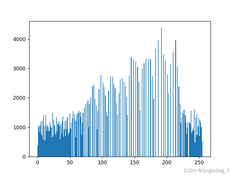
plt.hist(img.ravel(),256)
plt.show()

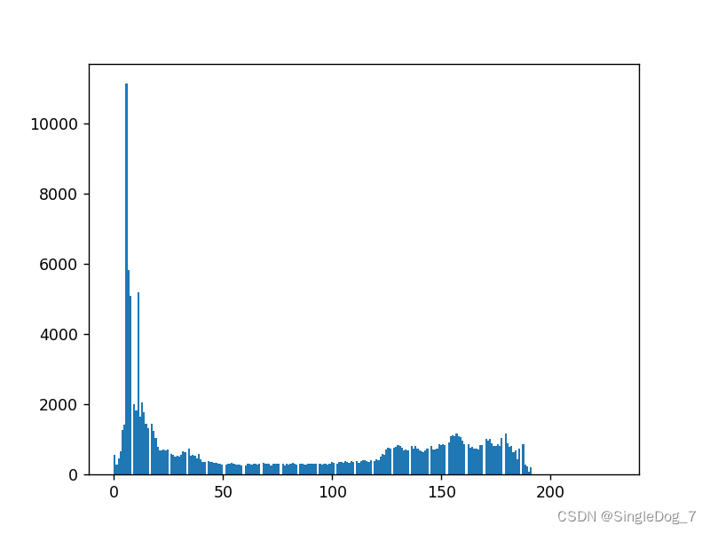
We will get a histogram similar to the above .

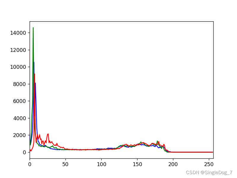
img =cv2.imread('cat.jpg')
print(img.shape)
color =('b','g','r')
for i,col in enumerate(color):
    histr = cv2.calcHist([img],[i],None,[256],[0,256])
    plt.plot(histr,color=col)
    plt.xlim([0,256])
plt.show()

  Use the above operation , You can get the line graph of three color channels ：

mask operation ：

Mask = Mask ？

mask = np.zeros(img.shape[:2],np.uint8)  # Create a black one with img Same size image 
print(mask.shape)
mask[100:200,100:367]=255      # Set up areas , Set the area to be saved to 255
cv_show('a',mask)

  You can get the following image ：

  Black areas represent masking , White areas indicate that ,

masked =cv2.bitwise_and(img,img,mask=mask)   # And operation , Not with mask and , It's two img And , Then only output the mask instead of 0 Part of 
cv_show('b',masked)

histr = cv2.calcHist([img],[0],mask,[256],[0,256])
plt.plot(histr,color='b')
plt.xlim([0,256])
plt.show()

Let's take a look at the changed line chart ：

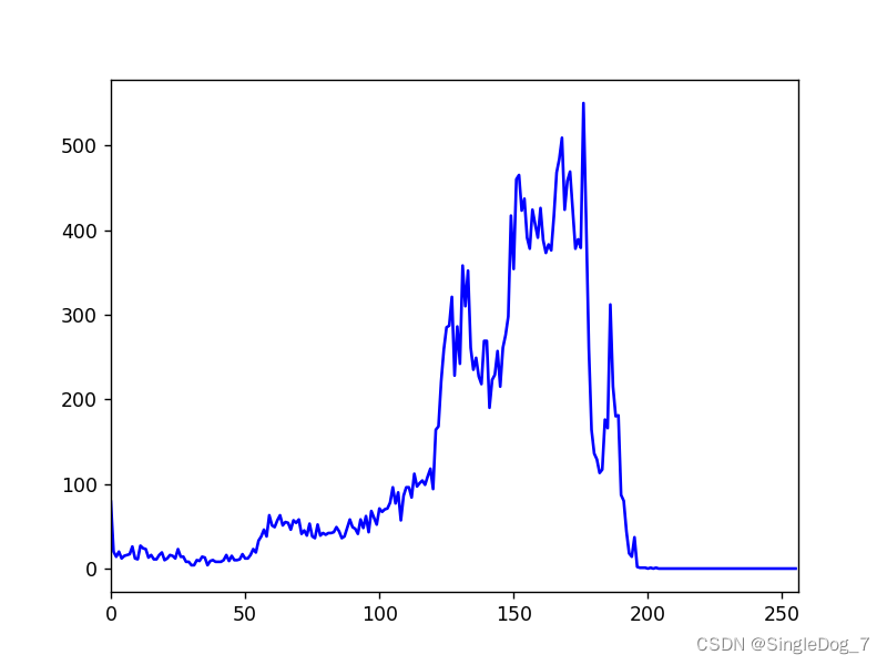
We will find it closer to the middle .

  equalization

Equalization process ： Histogram equalization ensures that the original size relationship remains unchanged in the process of image pixel mapping , That is, the brighter areas are still brighter , The darker ones are still darker , Just the contrast increases , Don't invert light and shade ; Ensure that the value range of the pixel mapping function is 0 and 255 Between . The cumulative distribution function is a single growth function , And the range is 0 To 1.

  The purpose of equalization is to increase image contrast ？

# equilibrium : Enhance image contrast ?
img1 =cv2.imread('dog.jpg',0)
plt.hist(img.ravel(),256)
plt.show()


equ=cv2.equalizeHist(img1)
plt.hist(equ.ravel(),256)
plt.show()

res=np.hstack((img1,equ))
cv_show('d',res)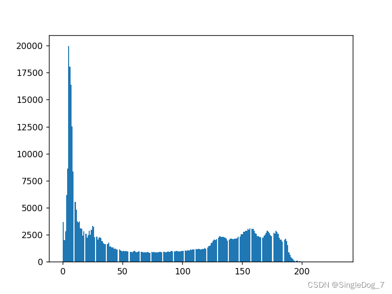

The first one is before the equalization operation , We will find that , Image histogram is more prominent , The second chapter is after the equalization operation , The image histogram will appear smoother .

  This is the comparison between before and after operation .

  Adaptive histogram equalization , Use block operation , The overall effect will be better , But the edge will be a little obvious blocky

# Adaptive histogram equalization ： Block ？ Cut both ways 
clahe =cv2.createCLAHE(clipLimit=2.0,tileGridSize=(8,8))    #clipLimit Clip limits    tileGridSize Tile grid size 
res_ = clahe.apply(img1)
res=np.hstack((img1,equ,res_))
cv_show('e',res)

Comparison of three pictures ：

The Fourier transform ：

# frequency domain ？ The stack ？ Change direction in time domain ？

# high frequency ： The grayscale components that change dramatically , The border
# Low frequency ： Change is slow

# low pass filter ： Keep only the low frequencies , Image blur
# High pass filter ： Keep only the high frequencies , Detail enhancement
#opencv in cv2.dft() and cv2.idft(), The input image needs to be converted into np.flota32 Format （ Time domain results ）
# The frequency of the results obtained is 0 It's going to be in the upper left corner , It's usually a shift to a central position , Can pass shift To achieve
#cv2.dft() The result returned is dual channel （ real , virtual ）, It usually needs to be converted into image format to display （0,255）

Fourier transform is the transformation of a function in space domain and frequency domain , The transformation from space domain to frequency domain is Fourier transform , From the frequency domain to the spatial domain is the inverse Fourier transform
Time domain and frequency domain ：

  frequency domain (frequency domain)
When analyzing a function or signal , Analyze the part related to frequency , Not the time related part , As opposed to the word time domain .
  Time domain
It describes the relationship between mathematical function or physical signal and time . For example, the time-domain waveform of a signal can express the change of signal with time . If you consider discrete time , A function or signal in the time domain , The values at each discrete time point are known . If continuous time is considered , Then the value of the function or signal at any time is known . When studying signals in the time domain , The oscilloscope is often used to convert the signal into its time-domain waveform .
  The transformation between the two
Time domain （ Signal as a function of time ） And frequency domain （ The signal as a function of frequency ） The transformation of is mathematically realized by integral transformation . Fourier transform can be directly used for periodic signals , For aperiodic signals, periodic expansion is needed , Using Laplace transform .
————————————————
Copyright notice ： This paper is about CSDN Blogger 「ShaneHolmes」 The original article of , follow CC 4.0 BY-SA Copyright agreement , For reprint, please attach the original source link and this statement .
Link to the original text ：https://blog.csdn.net/qq_33208851/article/details/94834614

  Here's a quote ShaneHolmes To explain the time domain and frequency domain .

img = cv2.imread('dog.jpg',0)
img_ = np.float32(img)

dft =cv2.dft(img_,flags=cv2.DFT_COMPLEX_OUTPUT)
dft_=np.fft.fftshift(dft)   # Convert the low-frequency value to the middle 

mag = 20*np.log(cv2.magnitude(dft_[:,:,0],dft_[:,:,1]))#20* It's for easy viewing 

plt.subplot(121),plt.imshow(img,cmap='gray')  #gary Report errors ？？？
plt.title('Input Image'),plt.xticks([]),plt.yticks([])
plt.subplot(122),plt.imshow(mag,cmap='gray')
plt.title('Magn'),plt.xticks([]),plt.yticks([])
plt.show()

# The low frequency is in the middle 

The low frequency is converted to the middle , Let's take a look at the image ：

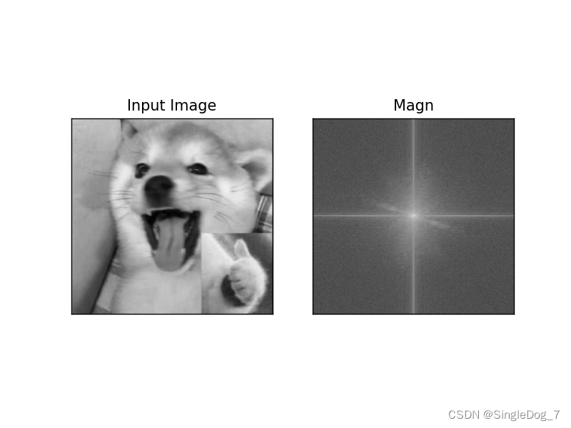
The low frequencies are concentrated in the middle , Near the white dot .

The inverse process realized by low-pass filtering

img = cv2.imread('dog.jpg',0)
img_ = np.float32(img)

dft =cv2.dft(img_,flags=cv2.DFT_COMPLEX_OUTPUT)
dft_=np.fft.fftshift(dft)   # Convert the low-frequency value to the middle 

row,cols = img.shape# Graphic shape Value size 
crow,cool = int(row/2),int(cols/2) # The location of the center point 

# Low pass filtering 
mask =np.zeros((row,cols,2),np.uint8)
mask[crow-30:crow+30,cool-30:cool+30]=1

#IDFT( The reverse process )
fshift = dft_*mask
f_shift = np.fft.ifftshift(fshift)
img_back = cv2.idft(f_shift)
img_back = cv2.magnitude(img_back[:,:,0],img_back[:,:,1])

plt.subplot(121),plt.imshow(img,cmap='gray')  #gary Report errors ？？？
plt.title('Input Image'),plt.xticks([]),plt.yticks([])
plt.subplot(122),plt.imshow(img_back,cmap='gray')
plt.title('Result'),plt.xticks([]),plt.yticks([])
plt.show()

It will make the color of the image softer , It will also make the image blurred

The inverse process of high pass filtering only needs to be changed mask Just go ：

# High pass filtering ：
mask =np.ones((row,cols,2),np.uint8)
mask[crow-30:crow+30,cool-30:cool+30]=0  # difference 

  It will make the details of the image more prominent . In addition, it is more convenient to process in the frequency domain , More efficient .