Machine learning library scikit learn (linear model, ridge regression, insert a column of data, extract the required column, vector machine (SVM), clustering)

• This article is from 《Python Data analysis goes from beginner to proficient 》- Edited by tomorrow Technology
• As the name suggests, machine learning is to make machines （ Computer ） Simulate human learning , Effectively improve work efficiency .Python Third party libraries provided Scikit-Learn A large number of mathematical models and algorithms are integrated , Make data analysis 、 Machine learning becomes simple and efficient .
• Because this book focuses on data processing and data analysis , Not machine learning , So for Scikit-Learn The related technologies of are only briefly explained , It mainly includes Scikit-Learn brief introduction 、 install , And the commonly used linear regression model least square regression 、 Ridge return 、 Support vector machine and clustering .

10.1 Scikit-Learn brief introduction

• Scikit-Learn（ abbreviation SKlearn） yes Python Third party modules for , It is well-known in the field of machine learning Python Module one , It encapsulates common machine learning algorithms , Including the return （Regression）、 Dimension reduction （Dimensionality Reduction）、 classification （Classfication） And clustering （Clustering） Four machine learning algorithms .Scikit-Learn It has the following characteristics .
• Simple and efficient data mining and data analysis tools .
• Enable everyone to reuse in complex environments .
• Scikit-Learn yes Scipy Module expansion , It's based on NumPy and Matplotlib Module based . Take advantage of these modules , It can greatly improve the efficiency of machine learning .
• Open source , use BSD agreement , Available for business .

10.2 install Scikit-Learn

• Scikit-Learn Installation requirements are as follows ：
• Python edition ： higher than 2.7
• NumPy edition ： higher than 1.10.2
• Scipy edition ： higher than 0.13.3
• If installed NumPy and Scipy, Then install Scikit-Learn The easiest way is to use pip Tool installation . The installation command is as follows ：

pip install -U scikit-learn -i https://pypi.tuna.tsinghua.edu.cn/simpl

• Here we need to pay attention to ： Try to choose installation 0.21.2 edition , Otherwise, running the program may cause error prompts because the module version is not suitable ——“ Can't find a module that only works ”.

10.3 Linear model

• Scikit-Learn A linear model has been designed for us （sklearn.linear_model）, Call directly in the program , Linear regression analysis can be easily realized without writing too much code . First, learn about linear regression analysis .
• In linear regression , Include only one independent variable and one dependent variable , And the relationship between them can be approximately expressed by a straight line , This kind of regression analysis is called univariate linear regression analysis ; If the linear regression analysis includes two or more independent variables , And the relationship between dependent variable and independent variable is linear , It's called multiple linear regression .
• stay Python in , Don't worry about the tedious mathematical process of solving linear regression , Use it directly Scikit-Learn Of linear_model Module can realize linear regression analysis .linear_model The module provides many linear models , Including least square regression 、 Ridge return 、Lasso、 Bayesian regression, etc . This section mainly introduces the least square method u to i Back to Heling .
• First, import. linear_model modular , The program code is as follows ：

from sklearn import linear_model

• Import linear_model After module , In the program, the correlation function can be used to realize linear regression analysis .

10.3.1 Least squares regression

• Linear review is one of the basic algorithms in data mining , The idea of linear regression is actually to solve a set of equations , Get the regression coefficient , But after attending the error term , There is a change in the solution of the equation , Generally, the least square method is used for calculation , So-called “ Mahayana and Hinayana ” It means square , The least square method is also called the least square sum , The aim is to minimize the sum of squares of errors , Make the predicted value infinitely close to the true value .
• linear_model Modular LinearRegression() Function is used to realize least square regression .LinearRegression() Function fitting a linear model with regression coefficients , Make real data and predicted data （ Estimated value ） The sum of the squares of the residuals between them is the smallest , Infinitely close to real data .LinearRegression() The function syntax is as follows ：

linear_model.LinearRegression(fit_intercept=True,normalize=False,copy_X=True,n_jobs=None)

• fit_intercept: Boolean value , Need to calculate intercept , The default value is True
• normalize： Boolean value , Whether standardization is needed , The default value is False, With the parameters fit_intercept of . When fit_intercept Parameter values for False when , This parameter will be ignored ; When fit_intercept Parameter values for True when , Then the regression quantity before regression X Normalize （ Standardization ） Handle , Subtract the mean , Divided by L2 norm （L2 Norm is the sum of the squares of the elements of a vector and then the square ）.
• copy_X: Boolean value , Choose whether to copy X data , The default value is True, If the value is False, Coverage X data .
• n_jobs： integer , representative CPU Audit of work efficiency , The default value is 1,-1 Means to follow CPU Consistency of nuclear numbers .coef_： Array or shape , Represents the regression coefficient of linear regression analysis .intercept_： Array , It means intercept .
• The main method ：
• fit(X,y,sample_weight=None): Fit linear model .
• predict(X): Use the linear model to return the prediction data .
• score(X,y,sample_weight=None): Returns the coefficient of certainty of the forecast R^2
• LinearRegression() Function call fit() Method to fit the array X、y, And the regression coefficients of the linear model are stored in its member variables coef_ Properties of the .

Intelligent prediction of house prices （01）

• Intelligent prediction of house prices , Suppose the area and price of a house are conceptually shown in the figure 10.2 Shown , Use LinearRegression() The function predicts an area of 170 The unit price of a square meter house .
  
• The program code is as follows ：

from sklearn import linear_model
import numpy as np
x=np.array([[1,56],[2,104],[3,156],[4,200],[5,250],[6,300]])
y=np.array([7800,9000,9200,10000,11000,12000])
clf = linear_model.LinearRegression()
clf.fit (x,y)    # Fit linear model 
k=clf.coef_      # Regression coefficient 
b=clf.intercept_ # intercept 
x0=np.array([[7,170]])
# By giving x0 forecast y0,y0= intercept +X value * Regression coefficient 
y0=clf.predict(x0) # Predictive value 
print(' Regression coefficient ：',k)
print(' intercept ：',b)
print(' Predictive value ：',y0)

 Regression coefficient ： [1853.37423313  -21.7791411 ]
 intercept ： 7215.950920245396
 Predictive value ： [16487.11656442]

10.3.2 Ridge return

• Ridge regression is based on least square regression , Add a pair of L2
  Norm constraint . Ridge regression is a kind of reduction method , Relative to imposing restrictions on the size of the regression coefficient . Ridge regression mainly uses linear_model Modular Ridge() Function implementation . The grammar is as follows ：

linear_model.Ridge(alpha=1.0, fit_intercept=True,normalize=False,copy_X=True,max_iter=None,tol=0.001,solver="auto",random_state=None)

• alpha: The weight .
• fit_intercept： Boolean value , Need to calculate intercept , The default value is True.
• normalize： The input sample features are normalized , The default value is False.
• copy_X： Copy or rewrite .
• max_iter: Maximum number of iterations .
• tol： Floating point numbers , Control the accuracy of the solution .
• solver： solver , Its values include auto、svd、cholesky、sparse_cg and lsqr, The default value is auto
• coef_: Array or shape , Represents the regression result of linear regression analysis .
• The main method
• fit(X,y): Fit linear model .
• predict(X)： Use the linear model to return the prediction data .
• Ridg() Function USES fit() Methods the regression coefficients of the linear regression model are stored in its member variables coef_ Properties of the .

Use ridge regression function to realize intelligent prediction of house prices （02）

• Use Ridg() Realize intelligent prediction of house prices , The program code is as follows ：

from sklearn.linear_model import Ridge
import numpy as np
x=np.array([[1,56],[2,104],[3,156],[4,200],[5,250],[6,300]])
y=np.array([7800,9000,9200,10000,11000,12000])
clf = Ridge(alpha=1.0)
clf.fit(x, y)
k=clf.coef_             # Regression coefficient 
b=clf.intercept_        # intercept 
x0=np.array([[7,170]])
# By giving x0 forecast y0,y0= intercept +X value * Slope 
y0=clf.predict(x0)      # Predictive value 
print(' Regression coefficient ：',k)
print(' intercept ：',b)
print(' Predictive value ：',y0)

 Regression coefficient ： [10.00932795 16.11613094]
 intercept ： 6935.001421210872
 Predictive value ： [9744.80897725]

10.4 Support vector machine

• Support vector machine （SVM） It can be used for supervised learning algorithm , It mainly includes classification 、 Regression and anomaly detection . The method of support vector classification can be extended to solve regression problems , This method is called support vector regression .
• This section introduces support vector regression functions ——LinearSVR() function .LinearSVR() Class is a function of support vector regression , Support vector regression is not only applicable to linear models , It can also be used to study the nonlinear relationship between data and features . Avoid multicollinearity problems , So as to improve the generalization performance , Solve high-dimensional problems , The grammar is as follows ：

sklearn.svm.LinearSVR(epsilon=0.0,tol=0.0001,C=1.0,loss='epsilon_insensitive',fit_intercept=True,intercept_scaling=1.0,dual=True,verbose=0,random_state=None,max_iter=1000)

• epsilon:float Type values , The default value is 0.0
• tol：float Type values , The standard value of terminating the iteration , The default value is 0.0001
• C：float Type values , Penalty parameter , The larger the parameter , The less regularization is used , The default value is 1.0
• loss：string Type values , Loss function , This parameter has the following two options ：epsilon_insensitive: The default value is , Insensitive to loss （ standard SVR） yes L1 Loss .squared_epsilon_insensitive: The square insensitive loss is L2 Loss .
• fit_intercept:boolean Type values , Whether to calculate the intercept of this model . If the setting is False, The intercept will not be used in the calculation （ That is, the data is expected to be in the middle ）. The default value is True.
• intercept_scaling：float Type values , When fit_intercept by True when , Instance vector x Turn into [x,self.intercept_scaling]. This is equivalent to adding a feature , This feature will be constant for all instances .
• dual：boolean Type values , Choose an algorithm to solve dual or primal optimization problems . When the setting value is True when , Dual problems can be solved ; When the setting value is False when , It can solve the original problem . The default value is True.
• verbose：int Type values , Open or not verbose Output , The default value is 0
• random_state：int Type values , Seed of random number generator , Used in data cleaning . The default value is None.
• max_iter：int Type values , The maximum number of iterations to apply . The default value is 0
• Two important attributes ：
  – coef_: Weight a feature , return array data type .
  – intercept_： Constant in decision function , return array data type .

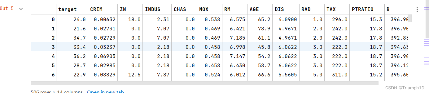
Boston house price forecast

• adopt Scikit-Learn Native data set “ Boston prices ”, Realize the house price forecast , The program code is as follows ：

from sklearn.svm import LinearSVR              #  Import linear regression class 
from sklearn.datasets import load_boston      #  Import and load Boston dataset 
from pandas import DataFrame                     #  Import DataFrame
boston = load_boston()                            #  Create and load Boston data objects 
#  Create Boston house price data as DataFrame object 
df = DataFrame(boston.data, columns=boston.feature_names)
df

df.insert(0,'target',boston.target)             #  Add price to DataFrame In the object 
df

data_mean = df.mean()                              #  Get the average value of each column 
data_std = df.std()                                 #  Obtain the standard deviation 
data_train = (df - data_mean) / data_std       #  Data standardization 
data_train

x_train = data_train[boston.feature_names].values       #  Characteristic data ,feature_names In the above figure, except target Values of other columns except column 
y_train = data_train['target'].values                      #  Target data 

It also uses the list method to directly extract the values of the required columns , such as data_train[[‘target’,‘ZN’]]…values Is to get target Column sum ZN Columns of data ;data_train[[‘target’：‘ZN’]]…values It's getting from targer To ZN There are three columns of data .

#%%
linearsvr = LinearSVR(C=0.1)                                  #  establish LinearSVR() object 
linearsvr.fit(x_train, y_train)                              #  Training models 
#  forecast , And restore the results 
x = ((df[boston.feature_names] - data_mean[boston.feature_names]) / data_std[boston.feature_names]).values
x

#  Add information column of predicted house price 
df[u'y_pred'] = linearsvr.predict(x) * data_std['target'] + data_mean['target'] # This is the code to restore the result 
df[['target','y_pred']] # Extract the real price and forecast price 

10.5 clustering

10.5.1 What is clustering

• Clustering is similar to classification , The difference is that the classification required by clustering is unknown , In other words, I don't know what kind of , But through a certain algorithm automatic classification . in application , Clustering is a process of classifying and organizing data that are similar in some aspects （ Simply put, it is to gather similar data ）, Its schematic diagram is shown in the figure 10.3 Sum graph 10.4 Shown .

• The main application fields of clustering are as follows .
• business ： Cluster analysis is used to find different customer groups , And depict the characteristics of different customer groups through purchase patterns .
• biological ： Cluster analysis is used to classify animals and plants and to classify genes , Acquire the understanding of the inherent structure of population .
• The insurance industry ： Cluster analysis identifies groups of insurance policy holders through a high average consumption , According to the type of residence 、 Value and geographical location to judge the real estate grouping of a city .
• Internet ： Cluster analysis is used to classify documents on the Internet .
• Electronic Commerce ： Clustering analysis is also a very important aspect in e-commerce website data mining , Cluster customers with similar browsing behavior by grouping , And analyze the common characteristics of customers , It can better help e-commerce companies understand their customers , Provide more appropriate services to customers .

10.5.2 clustering algorithm

• k-means Algorithm is a clustering algorithm , It is an unsupervised learning algorithm , The purpose is to group similar objects into a cluster . The more similar the objects in the cluster are , The better the clustering effect is .
• Traditional clustering includes partition methods 、 Hierarchical approach 、 Density based method 、 Grid based method and model-based method . This section focuses on the introduction k-means clustering algorithm , It is a typical method of division , It can also be called k Mean clustering algorithm . What is k Mean clustering and related algorithms .

1.k-means clustering

• k-means Clustering is also known as k Mean clustering , It is a famous algorithm of partition clustering , Because of its simplicity and efficiency, it has become the most widely used of all clustering algorithms .k Mean clustering is given a set of data points and the number of clusters needed k,k Specified by the user ,k The mean value algorithm divides the data into k In cluster .

2. Algorithm

• Random selection k Points as initial centroid （ The center of mass is the center of all points in the cluster ）, Then assign each point in the dataset to a cluster , In particular , Find the nearest center of mass for each point , And assign it to the cluster corresponding to the centroid . When this is done , The centroid of each cluster is updated to the average of all the points in the cluster . This process will be repeated until a termination condition is met . The termination condition can be any of the following .
• No, （ Or the minimum number ） Objects are reassigned to different clusters .
• No, （ Or the minimum number ） The cluster center changes again .
• The sum of the squares of the errors is locally minimum .
• Pseudo code ：

"""
 establish k Point as the starting center of mass , You can choose... At random （ Within the data boundary ）
 When the cluster allocation result of any point changes （ Initialize to True）
     For each data point in the dataset , Redistribute the center of mass 
         For every center of mass 
             Calculate the distance between the centroid and the data point 
         Assign data points to the nearest cluster 
     For each cluster , Calculate the mean of all points in the cluster and take the mean as the new centroid 
"""

• Through the above code introduction, I believe readers are right k-means Clustering algorithm has a preliminary understanding , And in the Python There is no need to write code manually to apply this algorithm , because Python Third-party module Scikit-Learn It has been written for us , It is much better in performance and stability than what I wrote , Just call it in the program , There is no need to build your own wheels .

10.5.3 Clustering module

• Scikit-Learn Of cluster The module is used for cluster analysis , This module provides many clustering algorithms , Here is the main introduction KMeans Method , The method is passed by k-means Clustering algorithm realizes clustering analysis .
• First, import. sklearn-cluster Modular KMeans Method , The program code is as follows ：

from sklearn.cluster import KMeans

• Next , You can use... In the program KMeans() The method .KMeans() The syntax of the method is as follows ：

KMeans(n_clusters=8,init='k-means++',n_init=10,max_iter=300,tol=1e-4,precompute_distances='auto',verbose=0,random_state=None,copy_x=True,n——jobs=None,algorithm='auto')

• n_cluster： integer , The default value is 8, Is the number of clusters generated , The resulting center of mass (centroid) Count .
• init： Parameter values for k-means++、random Or pass a numeric vector . The default value is k-means++.
  – k-means++： A special method is used to select the initial centroid so as to accelerate the convergence of the iterative process .
  – random： Random selection of initial centroid from training data . If you pass the array type , It should be shape(n_clusters,n_features) In the form of , And give the initial center of mass .
• n_init： integer , The default value is 10, The number of times the algorithm is run with different centroid initialization values .
• max_iter: integer , The default value is 300, Every time k-means The maximum number of iterations of the algorithm .
• tol： floating-point , The default value is 1e-4（ Scientific enumeration , namely 1 ride 10 Of -4 Power ）, Control the accuracy of the solution .
• precompute_distances： Parameter values for auto、True perhaps False. Used to calculate the distance in advance , Computing speed is faster when it takes up more memory .
  – auto： If the number of samples multiplied by the number of clusters is greater than 12e6（ namely 12 ride 10 Of 6 Power ）, Then the distance is not calculated in advance .
  – True： Always pre calculate the distance .
  – False： Never estimate the distance in advance .
• verbose: integer , The default value is 0, Verbose patterns .
• random_state： Integer or random array type . The generator used to initialize the center of mass （generator）. If the value is an integer , Then determine a seed (seed). The default value is NumPy The random number generator of .
• copy_x: Boolean type , The default value is True. If the value is True, Then the original data will not change ; If the value is False, It will directly modify the original data , And restore it when the function returns . But in the process of calculation, because of the addition and subtraction of the mean value of the data , So when the data comes back , There may be slight differences between the original data and the calculated data .
• n_jobs： integer , Specifies the number of processes used for the calculation . If the value is -1, Use all of CPU Carry out operations ; If the value is 1, Then parallel computation will not be carried out , This is convenient for debugging ; If the value is less than -1, It uses CPU The number of (n_cpus+1+n_jobs), for example n_jobs=-2, It uses CPU Number is total CPU Digital subtraction 1.
• algorithm: Express k-means Algorithm rule , Parameter values for auto、full or elkan, The default value is auto.
• Main attributes ：
• cluster_centers_: Returns an array of , Represents the mean vector of the classification cluster .
• labels_： Returns an array of , Indicates the category mark to which each sample data belongs .
• inertia_： Returns an array of , Represents the sum of the centers of each sample data from their nearest clusters .
• fit(X[,y]): Calculation k-means clustering .
• fit_predict(X[,y]): Calculate the cluster centroid and predict the category for each sample data .
• predict(X): Estimate the nearest cluster for each sample .
• score(X[,y])： Calculate the clustering error .

Cluster a set of data .

import numpy as np
from sklearn.cluster import KMeans
X=np.array([[1,10],[1,11],[1,12],[3,20],[3,23],[3,21],[3,25]])
kmodel = KMeans(n_clusters = 2)      # call KMeans Method to realize clustering （ Two types of ）
y_pred=kmodel.fit_predict(X)         # Forecast category 
print(' Forecast category ：',y_pred)
print(' Mean vector of classification cluster ：','\n',kmodel.cluster_centers_)
print(' Category marker ：',kmodel.labels_)

 Forecast category ： [1 1 1 0 0 0 0]
 Mean vector of classification cluster ： 
 [[ 3.   22.25]
 [ 1.   11.  ]]
 Category marker ： [1 1 1 0 0 0 0]

10.5.4 Clustering data generator

• 10.5.3 Section lists a simple clustering example , But the clustering effect is not obvious . This section generates test data of special Clustering Algorithm , It can better interpret the clustering algorithm , Show the clustering effect .
• Scikit-Learn Of make_blobs() Method is used to generate test data of clustering algorithm , Intuitively speaking ,make_blobs() Methods can be based on the number of features specified by the user 、 Number of center points 、 Range, etc. generate several types of data , These data can be used to test the effect of clustering algorithm .
• make_blobs() The syntax of the method is as follows ：

sklearn.datasets.make_blobs(n_samples=100,n_features=2,centers=3,cluster_std=1.0,center_box=(-10.0,10.0),shuffle=True,random_state=None)

• n_samples： Total number of samples to be generated .
• n_features： The number of features per sample .
• centers: Number of categories .
• cluter_std: Variance of each category , for example , Generate two types of data , One has a larger variance than the other , Can be cluster_std Set to [1.0,3.0].

Generate test data for clustering

• Generate data for clustering （500 Samples , Each sample has two characteristics ）, The program code is as follows ：

from sklearn.datasets import make_blobs
import matplotlib.pyplot as plt
x,y = make_blobs(n_samples=500, n_features=2, centers=3)

• Next , adopt KMeans() Methods cluster the test data , The program code is as follows ：

from sklearn.cluster import KMeans
y_pred = KMeans(n_clusters=4, random_state=9).fit_predict(x)
plt.scatter(x[:, 0], x[:, 1], c=y_pred)
plt.show()

• Run the program , The effect is as follows ：
  
• From the analysis results ： Similar data come together , Divided into 4 Pile up , That is to say 4 class , And display in color , It looks clear and intuitive .

10.6 Summary

• Through the study of this chapter , Be able to understand machine learning Scikit-Learn modular , This module contains a large number of algorithm models , This chapter introduces only a few common models combined with quick examples , Strive to make it easy for readers to get started , Quickly understand the usage of related models , And lay a good foundation for later learning data analysis and prediction projects .