Paper reading: u-net++: redesigning skip connections to exploit multiscale features in image segmentation

Address of thesis ： https://arxiv.org/pdf/1912.05074.pdf

The most advanced medical image segmentation model is U-Net And full convolution network (FCN) A variation of the . Despite the success of these models , But they have two limitations ：（1） The optimal depth of is unknown a priori , Need extensive architecture search or integration of different depth models ;（2） Jumping connections impose unnecessary restrictive fusion schemes , It can only be aggregated on the same scale feature map of encoder and decoder sub networks . To overcome these two limitations , We propose a new semantic and instance segmentation neural structure U-Net++, adopt （1） With different depths u Effective integration of network , Partially shared encoder , At the same time, we use deep supervised collaborative learning ;（2） Redesign jump connection , Aggregate features of different semantic scales on the decoder subnet , Form a highly flexible feature fusion scheme ;（3） A pruning scheme is designed to speed up U-Net++ The reasoning speed of . We use six different medical image segmentation dataset pairs U-Net++ An assessment was made , It covers a variety of imaging methods , Such as computed tomography (CT)、 MR imaging (MRI) And electron microscope (EM), And prove that （1）U-Net++ It is always better than the baseline model in the semantic segmentation tasks of different data sets and backbone architectures ;（2）U-Net++ It improves the segmentation quality of objects with different sizes —— For fixed depth U-Net Improvement ;（3）Mask RCNN++( Use U-Net++ Designed mask R-CNN) It is better than the original mask in the task of instance segmentation R-CNN; and （4） clipped U-Net++ The model achieves significant acceleration , It only shows moderate performance degradation . Our implementation and pre training model can be found in https://github.com/MrGiovanni/U-NetPlusPlus Found on the .

key word ： Neuronal structure segmentation 、 Liver segmentation 、 Cell segmentation 、 Nuclear division 、 Brain tumor segmentation 、 Pulmonary nodule segmentation 、 Medical image segmentation 、 Semantic segmentation 、 Instance segmentation 、 In depth Supervision 、 Model pruning .

1、 INTRODUCTION

Codec networks are widely used in modern semantic and instance segmentation models [1]、[2]、[3]、[4]、[5]、[6]. Their success is largely due to their jumping connection , Combine deep 、 semantics 、 Coarse grained feature map from decoder sub network shallow , low 、 Fine grained feature map from encoder sub network , It has been proved to be effective in recovering the fine-grained details of the target object [7],[8],[9] Even in complex backgrounds [10],[11]. Jumping connection also plays a key role in the success of instance level segmentation model , Such as [12],[13], The idea is to segment and distinguish each instance of the desired object .

However , These encoders for image segmentation - Decoder architecture has two limitations . First , Encoder - The optimal depth of the decoder network can vary from application to application , This depends on the difficulty of the task and the amount of marker data available for training . A simple method is to train models with different depths , Then in reasoning time [14]、[15]、[16] During the integration of the generated model . However , From a deployment perspective , This simple method is inefficient , Because these networks do not share a common encoder . Besides , After independent training , These networks don't enjoy multitasking [17],[18] The benefits of . secondly , In coding - The design of hop connections used in decoder networks is an unnecessary limitation , It requires the fusion of feature mapping of encoder and decoder with the same scale . Although as a natural design and eye-catching , But the same scale feature maps from decoder and encoder networks are semantically different , And there is no reliable theory to ensure that they are the best match for feature fusion .

In this paper , We proposed U-Net++, A new general image segmentation architecture , Designed to overcome the above limitations . Pictured 1(g) Shown ,U-Net++ By different depths u Network composition , Its decoder connects intensively with the same resolution through a redesigned hop connection . stay U-Net++ The architectural changes introduced in have the following advantages . First ,U-Net++ It is not easy to choose the network depth , Because it embeds different depths of u Type net . All of these u-nets Some share an encoder , And their decoders are intertwined . By training under deep supervision U-Net++, All composed U-Net Be trained at the same time , And benefit from shared image representation . This design not only improves the overall segmentation performance , And you can also prune the model during reasoning . secondly ,U-Net++ Not subject to unnecessary restrictive jump connections , In these connections , Only feature maps of the same scale from encoder and decoder can be fused . stay U-Net++ The redesigned hop connection introduced in presents characteristic graphs of different scales on the decoder node , The aggregation layer is allowed to decide how the various feature maps carried along the hop connection should be fused with the decoder feature map , Composed at the same resolution U-Net parts . We've been 6 Widely evaluated on segmented datasets and multiple backbones of different depths U-Net++. Our results show that , Driven by redesigned jump connections and depth supervision U-Net++, It can significantly improve the performance in semantics and instance segmentation . And classic U-Net Architecture compared to ,U-Net++ The significant improvement of is attributed to the advantages provided by the redesigned hop connection and extended decoder , Together, they enable image features to gradually converge in horizontal and vertical Networks .

All in all , We have made the following five contributions ：

1. We are U-Net++ A built-in different depth U- Network integration , It improves the segmentation performance of objects of different sizes —— For fixed depth U-Net Improvement ( see II-B section ).
2. We redesigned U-Net++ Jump connection in , Enable the decoder to flexibly fuse features —— That's right U-Net Improvement of restrictive jump connection in , The latter only requires feature map fusion of the same scale ( see II-B section ).
3. We designed a program to trim a trained U-Net++, Speed up their reasoning , While maintaining its performance ( See the first IV-C section ).
4. We found that , At the same time, training is embedded in U-Net++ Multi depth in architecture U-Nets Stimulus composition U-Net Collaborative learning between , It is more isolated than training the same structure alone U- Get better performance ( see IV-D Festival sum V-C section ).
5. We showed U-Net++ Scalability for multiple backbone encoders , And further apply it to various medical imaging modes , Include CT、MRI And electron microscope ( see IV-A Festival sum IV-B section ).

2、 PROPOSED NETWORK ARCHITECTURE: U-Net++

chart 1 Shows U-Net++ Is how from the original U-Net Evolved . Hereunder , We first track this evolution , Inspired the right to U-Net++ The needs of , Then explain its technology and implementation details .

2.1 Motivation behind the new architecture

We have done a comprehensive ablation study to study different depths u-nets Performance of ( chart 1(ad)). So , We used three relatively small data sets , namely Cell, EM, and Brain Tumor( See page for details III-A section ). surface 1 These results are summarized . For the segmentation of cells and brain tumors , A shallow network (U-NetL3) Performance is better than depth U-Net. On the other hand , about EM Data sets , Deeper U-Net Net is always better than shallow , But the performance gain is only limited . Our experimental results show two key findings ：1) A deeper cellular network is not always better ,2) The optimal depth of the architecture depends on the difficulty and size of the data set at hand . Although these findings may encourage automatic neural structure search , But this method suffers from limited computing resources [19]、[20]、[21]、[22]、[23] Obstacles . in addition , We propose an integration architecture , It will have different depths U-Net Combine into a unified structure . We call this architecture $U-Ne{t}^e$（ chart 1(e)）. We do this by creating a set for each U-Net Define a separate loss function to train $U-Ne{t}^e$, namely $X^{0,j},j\in \{1,2,3,4\}$. Our depth supervision scheme is different from the depth supervision commonly used in depth image classification and image segmentation Networks ; stay [24]、[25]、[26]、[27] in , Add to the node along the decoder network , namely $X^{4-j,j},j\in \{0、1、2、3、4\}$, And we apply it to $X_{0,j},j\in \{1、2、3、4\}$. In reasoning , Each of the sets U-Net The output of is averaged .

The integration architecture outlined above ($U-Ne{t}^e$)【$U-Ne{t}^e$ For each level feature map Have designed decoders , And implemented feature map Long connection with multiple decoders at the same level 】 It's good for knowledge sharing , Because all in the integration U-Nets All share the same encoder , Even if they have their own decoder . However , This architecture still has two disadvantages . First , The decoder is disconnected —— Deeper U-Net Not to the shallower in the integration U-Net The decoder of provides supervisory signals . secondly , stay U-Nete The common design of jump connections used in is unnecessary constraints , The network is only required to combine the characteristic map of the decoder with the characteristic map of the same scale from the encoder . Although as a natural design and eye-catching , However, there is no guarantee that the feature map with the same scale is the best match for feature fusion .

To overcome these limitations , We from $U-Ne{t}^e$ Deleted the original jump connection , And connect every two adjacent nodes in the integration , Thus, a new architecture is produced , We call it U-Net+( chart 1(f))【$U-Ne{t}^e$ For each level feature map Have designed decoders , And realize the short connection between multiple decoders of the same level 】. Due to the new connection scheme ,U-Net+ Connected to disjoint decoders , Make gradient back-propagation from deeper decoder to shallower corresponding decoder .U-Net+ By combining each node in the decoder with the aggregation of all feature maps calculated in the shallower stream , The unnecessary restrictive behavior of jumping connection is further relaxed . Although the limitation of using aggregate feature mapping on the decoder node is much smaller than that of the same scale feature mapping from the encoder , But there is still room for improvement . We further suggest that U-Net+ Use dense connections in , This led to our final architectural proposal , We call it U-Net++( chart 1(g)).

In the case of dense connections , Each node in the decoder not only has the final aggregated feature graph , It also shows the intermediate aggregation feature map and the original same scale feature map of the encoder . therefore , The aggregation layer in the decoder node can learn to use only the encoder feature map of the same scale or collect the input feature map . And $U-Ne{t}^e$ Different ,U-Net+ and U-Net++ In depth supervision is not required , However , As we will describe later , Deep supervision enables the model to prune during reasoning , Significant acceleration , The performance is only slightly reduced .

2.2 Technical details

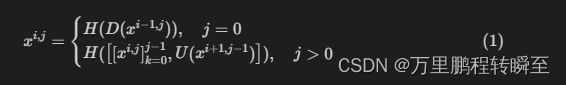
1. Network connectivity ： set up $x^{i,j}$ Represents a network node ( given layer)$X^{i,j}$ Output , among i Represents the lower sampling layer along the encoder ,j Represents the convolution layer of dense blocks connected along the jump . from $x^{i,j}$ The feature mapping stack represented is evaluated as a formula 1 Shown
   
   $$ x^{i,j}=
   \begin{cases}
   H(D(x^{i-1,j})) ,\quad j=0 \
   H(\big[[x^{i,j}]_{k=0}{j-1}, U(x^{i+1,j-1})\big]), \quad j>0
   \end{cases}

\tag{1}
$$

• • among , function H() It's a convolution operation + An activation function ,D() and U() Represents the lower sampling layer and the upper sampling layer respectively ,[] Represents the connection layer . Basically , Pictured 1(g) Shown ,j=0 The node of stage receives only one input from the previous layer of the encoder ;j=1 The node of the stage receives two inputs , All from the encoder sub network , But two consecutive levels ;j>1 The node of level receives j+1 Input , among j Input is the same jump connection before j Output of nodes , The first j+1 The first input is the upsampling output of the hop down connection . The reason why all previous feature maps accumulate and reach the current node is , We use a dense convolution block on each hop connection .

2. In depth Supervision ： We are U-Net++ In depth supervision is introduced . So , We're at the node $X^{0,1}$、$X^{0,2}$、$X^{0,3}$ and $X^{0,4}$ An... Is appended to the output of 1×1 Convolution , And then a sigmid Activation function , among C yes s The number of classes in the dataset . then , We define a hybrid partition loss , Including pixel level cross entropy loss and soft dice Each semantic scale of coefficient loss . The mixed loss can be provided by two loss functions ： Smooth gradient and deal with class imbalance [28],[29]. In Mathematics , The mixing loss is defined as ：
   $$crossentropyloss()+diceloss()$$

3. Mold Trim ： Through in-depth supervision , Model pruning can be realized . Due to in-depth supervision ,U-Net++ It can be deployed in two operation modes ：1) Integration mode ： Segmentation segmentation result collection , Then average ;2) Trim mode ： Split output selection has only one split Branch , Selection determines the degree of model trimming and speed gain . chart 2 It shows the branch pruning structure with different complexity . say concretely , take $X^{0,4}$ The segmentation result of does not lead to pruning , And take $X^{0,4}$ The segmentation result of will lead to the maximum pruning of the network .
   

3、EXPERIMENTS

3.1 Datasets

surface 2 Summarizes the... Used in this study 6 Biomedical image segmentation dataset , It includes the lesions of the most commonly used medical imaging methods / organ , Including microscope 、 Computed tomography (CT) And MRI (MRI).

1） Electron Microscopy(EM)： The data set is composed of EM Segmentation challenges [30] Provide , As ISBI 2012 Part of . The dataset includes 30 Zhang image （512×512 Pixels ）, Serial sectioning transmission mirror from the first instar larvae of Drosophila melanogaster (VNC). Refer to the picture 3 Examples in , Each image has corresponding cells （ white ） And cell membrane （ black ） Real segmentation map of the ground . The marked images are divided into training （24 Zhang image ）、 verification （3 Zhang image ） And testing （3 Zhang image ） Data sets . Training and reasoning are based on 96×96 Of patches Accomplished , these patches Select the overlapped half by sliding the window patches size . say concretely , In the process of reasoning , We aggregate across... By voting in overlapping areas patches The forecast .

2） Cell： The data set is through Cell-CT Imaging system [31] To obtain the . Two trained experts manually segment overlapping images , Therefore, each image in the dataset has two binary cell masks . In our experiment , We chose 354 A subset of images , They have the highest level of consistency between two expert commentators . Then divide the selected image into training （212 Zhang image ）、 verification （70 Zhang image ） And testing （72 Zhang image ） A subset of .

3）Nuclei： The data set is composed of 2018 The annual data science bowl segmentation challenge provides , from 670 Zhang comes from different modes （ Bright field and fluorescence ） Segmentation nuclei Image composition . This is the only dataset with instance level annotation used in this work , Each of them nuclei Mark with different colors . Images are randomly assigned to a training set （50%）、 A validation set （20%） And a test set （30%） in . then , We use the sliding window mechanism to extract 96×96 Of patch,32 Pixel strides are used to train and validate models ,1 Pixel strides are used for testing .

4） Brain Tumor： The data set is composed of BraTS2013[32,34]. Provide . To facilitate comparison with other methods , Model USES 20 High level (HG) and 10 A low level (LG) Training , For all patients Mr Image processing Flair、T1、T1c and T2 scanning , Get... Together 66,348 A slice . We rescale the slice to 256×256 To further preprocess the data set . Last , Available in the dataset 30 Patients were randomly divided into 5 times , Every 5 Times all come from 6 Images of patients . then , We randomly assign these five folded files to a training set （3 times ）、 A validation set （1 times ） And a test set （1 times ） in . There are four different labels for data ： Necrosis 、 edema 、 Non enhanced tumor and enhanced tumor . stay BraTS2013 after ,“ complete ” The evaluation is done by treating all four tags as positive , Treat other tags as negative .

5）Liver： The data set is composed of MICCAI 2017LiTS Challenges provide , Include 331 Time CT scanning , We divide it into training （100 Famous patients ）、 verification （15 Patients ） And testing （15 Patients ） A subset of . Real segmentation of the ground provides two different labels ： Liver and lesions . In our experiment , We only think that the liver is positive , Others are feminine .

6）Lung Nodule： The data set is provided by the lung image database alliance image collection center （ Lithium ion ）[33] Provide , from 7 Home academic center and 8 Collected by medical imaging companies 1018 Case composition .6 Cases with ground truth issues were confirmed and deleted . The remaining cases were divided into training （510）、 verification （100） And testing （408） Set . Each case is three-dimensional CT scanning , Nodules are marked 3 Dimensional binary mask . We resample the volume to 1-1-1 spacing , Then extract around each nodule 64×64×64 Of crop. These three dimensions crop Used for model training and evaluation .

3.2 Baselines and implementation

For comparison , We use the original U-Net[35] And customized wide U-Net The architecture is used for 2D Split task , Use V-Net[28] And customized wide V-Net The architecture is used for 3D Split task . We choose U-Net( or V-Net be used for 3D), Because it is a common performance baseline for image segmentation . We also designed a wide U-Net( Or three-dimensional wide V-Net), The number of parameters is similar to our proposed architecture . This is to ensure that the performance gain generated by our architecture is not just due to the increase in the number of parameters . surface 3 Detailed U-Net and wide U-Net Architecture . We further compare U-Net++ And U-Net+ Performance of , This is our intermediate architecture proposal . The number of cores in the intermediate node is shown in table 3.

Our experiment is in Keras Implemented in （backend by tensorflow）. We use on validation sets early-stop Mechanism , To avoid over fitting , And use Dice and IoU Evaluate the results . Other measurement indicators , Such as pixel level sensitivity 、 Specificity 、F1 and F2 fraction , And statistical analysis can be found in the appendix a Section .Adam As an optimizer , The learning rate is 3e-4.U-Net+ and U-Net++ Are made of primitive U-Net Architecture built . All experiments used three NVIDIA titanX(Pascal)gpu, Everyone with a 12GB Memory .

4、RESULTS

4.1 Semantic segmentation results

surface 4 Comparison of the U-Net、wide U-Net、U-Net+ and U-Net++ Quantitative parameters and segmentation results . As I saw before ,wide U-Net Your performance is always better than U-Net. This improvement is attributed to wide U-Net More parameters in . stay neuronal structure（↑0.62±0.10,↑0.55±0.01）,cell（↑2.30±0.30,↑2.12±0.09）,nuclei（↑2.00±0.87,↑1.86±0.81）,liver（↑2.62±0.09,↑2.26±0.02）, and lung nodule（↑5.06±1.42,↑3.12±0.88） Split all 6 In this task , Units without in-depth supervision ++ stay U-Net And width U-Net Have achieved remarkable IoU gain . The use of in-depth monitoring and average voting has further improved U-Net++, send IoU Improved up to 0.8 percentage . say concretely ,neuronal structure and lung nodule Segmentation benefits most from in-depth supervision , Because they are EM and CT The slices appear at different scales . However , In depth monitoring can only be slightly effective for other data sets at most . chart 3 It describes U-Net、wide U-Net and U Net++ Qualitative comparison between the results .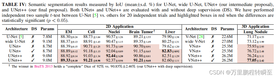

We further studied U-Net++ Extensibility for semantic segmentation , By applying the redesigned jump connection to modern CNN framework ：vgg-19[36]、resnet-152[8] and densenet-201[9]. say concretely , We add a decoder subnet , Convert each of the above architectures into U-Net Model , Then use the redesigned U-Net++ Connection replaced U-Net Pure jump connection of . For comparison , We also used the above backbone architecture to train U-Net and U-Net+. For a comprehensive comparison , We used EM、 cells 、 nucleus 、 Brain tumor and liver segmentation data set . Pictured 4 Shown ,U-Net++ The performance is always better than U-Net and U-Net+. adopt 20 trials , We went further to U-Net、U-Net+ and U-Net++ Each pair of is subjected to independent double samples t Statistical analysis of tests . Our results show that ,U-Net++ It's an effective , Unrelated to the trunk U-Net Expand . In order to facilitate reproducibility and model reuse , We have released U-Net、U-Net+ and U-Net++ The implementation of the 1.

4.2 Instance segmentation results

Instance segmentation includes the segmentation and differentiation of all object instances ; therefore , More challenging than semantic segmentation . We use Mask R-CNN[12] As the baseline model of instance segmentation .Mask R-CNN Using feature pyramid network (FPN) As the backbone , Generate targets on multiple scales proposal, Then output the collected data through a dedicated split Branch proposal Output split mask . We changed it MaskR-CNN, With redesigned U-Net++ Ordinary jump connection . We call this model Mask R-CNN++. We used... In the experiment resnet101 As Mask R-CNN The backbone of .

surface 5 Comparison of the Mask R-CNN And Mask R-CNN++ For the division of nuclei . We chose the nuclear dataset because multiple nucleolar instances can appear in one image , under these circumstances , Each instance is annotated with different colors , So mark it as a different object . therefore , This data set is applicable to semantic segmentation that regards all verification cases as foreground classes , It is also applicable to the segmentation of instances that separate each core . As shown in the table V Shown ,Mask RCNN++ Better than the original ,IoU Added 1.82 branch （93.28% to 95.10%）,Dice Added 3.45 branch （87.91% to 91.36%）, The ranking score has increased 0.013 branch （0.401-0.414）. In order to correctly understand this performance , We also trained one U-Net and U-Net++ Model , To use the resnet101 The backbone performs semantic segmentation . As shown in the table V Shown ,Mask R-CNN The model has higher segmentation performance than the semantic segmentation model . Besides , As expected ,U-Net++ Better than in semantic segmentation U-Net.

4.3 Model pruning

once U-Net++ Be trained , In reasoning , depth d The decoder path of is completely independent of depth d+1 Decoder path of . therefore , Due to the introduction of in-depth supervision , We can completely delete the decoder , At depth d+1, At depth d Get trained U-Net++ The lighter version of . This pruning can significantly reduce reasoning time , But the segmentation performance may be reduced . therefore , The level of pruning should be determined by evaluating the performance of the model on the validation set . We studied the graph 5 in U-Net++ Reasoning speed and Iou Balance . We use U-Net++$L^d$ Expressing depth d clipped U-Net++（ As shown in the figure 2）. As shown in the figure ,U-Net++$L^3$ An average decrease of 32.2% Reasoning time of , Less 75.6% Memory footprint , and IoU Only reduced 0.6 A little bit . More aggressive pruning further reduces inference time , But at the cost of significant degradation . what's more , Because the computer cost of the existing deep convolution neural network model is high , Therefore, computer-aided diagnosis of mobile devices (CAD) Have an important impact .

4.3 Embedded vs. isolated training of pruned models

Theoretically ,U-Net++$L^d$ There are two ways to train ：1) Embedded training is complete U-Net++ model training , Then trim the depth d get U-Net++$L^d$,2) Isolated training U-Net++$L^d$ Train in isolation without any interaction with deeper encoder and decoder nodes . Pictured 2 Shown , Embedded training of a sub network includes training all graph nodes through in-depth supervision （ Yellow and gray ingredients ）, But we only use yellow subnets during reasoning . by comparison , Isolated training involves removing grey nodes from the graph , Training and testing based only on the Yellow subnet .

We compared the graph 6 Different levels of U-Net++ Pruning isolation and embedded training program . We found that ,U-Net++$L^d$ Embedded training can produce higher performance models than training the same architecture alone . When the whole U-Net++ Be trimmed to U-Net++$L^1$ when , The advantages observed under aggressive pruning are more obvious . especially , For liver segmentation U-Net++$L^1$ Embedded training is more than isolated training 5 branch . This discovery shows that , Monitoring signals from deep downstream can train shallower models with higher performance . This discovery is also related to knowledge distillation , That is, the knowledge learned by a deep teacher online is learned by a shallow student online .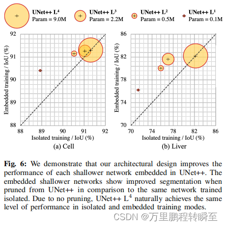

5. DISCUSSIONS

5.1 Performance analysis on stratified lesion sizes

chart 7 Comparison of the U-Net and U-Net++ Segmentation of brain tumors of different sizes . To avoid confusion in the diagram , We divide tumors by size 7 Kind of . As shown above ,U-Net++ The performance in all barrels is always better than U-Net. We are also based on 20 Different experiments were carried out on each barrel t Test to measure the significance of improvement , obtain 7 There are 5 Species have statistical significance (p<0.05).U-Net++ The ability to segment tumors of different sizes is attributed to its built-in u-nets Integrate , It supports image segmentation of multiple networks .

5.2 Feature maps visualization

In the second section II-A In the festival , We explained that the redesigned jump connection enables the semantic rich decoder feature map to be fused with the feature map of different semantic scales from the middle layer of the architecture . In this section , We will illustrate the advantages of our redesigned jump connection by visualizing the intermediate feature mapping .

chart 8 It shows the brain tumor image jumping along the top ( namely $X_{0,i}$) Early stage 、 Representative characteristics of intermediate and late layers . By averaging all the characteristic graphs of the first floor , Get the representative characteristic diagram of this layer . The other thing to note is that , chart 8 The architecture on the left uses only the decoder layer attached to the deepest ($X_{0,4})Training\; on\; the\; loss\; function\; ,\; Diagram8The\; structure\; on\; the\; right\; is\; trained\; through\; in-depth\; supervision\; .\; Please\; note\; that\; ,\; These\; feature\; mappings\; are\; not\; the\; final\; output\; .\; We\; attach\; an\; extra\; at\; the\; top\; of\; each\; decoder\; Branch1\times 1Convolution\; layer\; to\; form\; the\; final\; segmentation\; .\; We\; observed\; that\; ,U-NetThe\; output\; of\; the\; middle\; tier\; of\; is\; semantically\; different\; ,\; And\; forU-Net+andU-Net++The\; output\; of\; is\; gradually\; formed\; .U-NetNodes\; in$X_{0,0} The output of has undergone a slight conversion （ There are few convolution operations ）, and $X_{1,3}Output\; ,\; namely$X_{0,4} The input of , Almost every transformation learned through the network （4 Next sampling and 3 Upper sampling stage ）. therefore ,$X_{0,0}and$X_{1,3} There is a big gap between the presentation ability of . therefore , Simply connect $X_{0,4}and$X_{1,3} The output of is not an optimal solution . by comparison , stay U-Net+ and U-Net++ The redesigned jump connection in helps to refine the segmentation results step by step . We're in the appendix B The learning curve of all six medical applications is further shown in this section , Show in U-Net++ Adding dense connections to can promote better optimization , And achieve lower verification loss .

5.3 Collaborative learning in U-Net++

Collaborative learning refers to training multiple classifier heads of the same network on the same training data at the same time . The study found that , It can improve the depth of Neural Networks [37] Generalization ability .U-Net++ By aggregating multi depth networks and monitoring segmentation headers from each constituent network , It naturally embodies collaborative learning . Besides , Split head , For example, figure 2 Medium $X_{0,2}, From strong to strong （label Loss ） gentle （ The loss of propagation from adjacent deeper nodes ） Receive gradient in supervision . therefore , Shallow networks improve their segmentation （ chart 6）, And provide more information representation for deeper corresponding Networks . Basically , stay U-Net++ in , Deeper and shallower networks regulate each other through collaborative learning . Training a multi depth embedded network together is more conducive to segmentation than training an isolated network alone , This is in the IV-D It is obvious in section .U-Net++ Its embedded design makes it easy to carry out auxiliary training 、 Multi task learning and knowledge distillation 、[17]、[38]、[37]

6. RELATED WORKS

below , We will review the jump connection with the redesign 、 Work related to feature aggregation and in-depth supervision , These are the main components of our new architecture .

6.1 Skip connections

Skip Connect first in Long wait forsomeone [39] Was introduced into the groundbreaking work of , They proposed a full convolution network for semantic segmentation (FCN). Not long after , On the basis of jump connection , Ronnberg et al [35] A method for semantic segmentation of medical images is proposed U-Net framework . However ,FCN and U-Net The architecture of is different from how the up sampled decoder feature map is fused with the feature map of the same scale from the encoder network .FCN[39] Feature fusion using summation , and U-Net[35] Connect these features , Then apply convolution and nonlinearity . Jump connections help restore full spatial resolution , Make the method of complete convolution suitable for semantic segmentation [40],[41],[42],[43]. Jumping connections are further applied to modern neural structures , Like the residual network [8]、[44] And dense networks [9], Promote gradient flow , It improves the overall performance of the classification network .

6.2 Feature aggregation

The exploration of hierarchical characteristics of aggregation is a research topic in recent years .Fourure wait forsomeone .[45] Put forward GridNet, This is a codec architecture , Among them, feature mapping is connected by grid , Several classic segmentation architectures are generalized . Even though GridNet Contains multiple inputs with different resolutions , It lacks an upper sampling layer between skipping connections ; therefore , It doesn't mean U-Net++.Full-resolution residual networks (FRRN)[46] A two-stream System , The full resolution information is carried in one stream , Context information is carried in another pooled stream . stay [47] in , Two improved FRRN edition , namely 28.6M Increment of parameter MRRN and 25.5M Parameter density MRRN. However , these 2D The number of parameters of the architecture is similar to our 3D VNet++ be similar , Parameter is 2D U-Net++ Three times ; therefore , Simply upgrade these architectures to 3D The method may not be applicable to general 3D Volume medical imaging applications . What we want to pay attention to is , We redesigned the dense skip connection with MRRN Used in completely different ,MRRN It consists of a common residual flow . Besides , take MRRN The design of is applied to other backbone encoders and meta frameworks , Such as Mask R-CNN[12], Also inflexible .DLA2[48] In terms of topology, it is equivalent to our intermediate architecture U-Net+( chart 1(f)), Connect the characteristic images with the same resolution in sequence , Unlike U-Net Long hop connection used in . Our experimental results show that , Through dense connection of layers ,U-Net++ Than U-Net+/DLA It has higher segmentation performance （ See table 4）.

6.3 Deep supervision

He[8] People think , The depth of the network d It can be used as a regularizer .Lee wait forsomeone [27] prove , The deep supervision layer can improve the learning ability of the hidden layer , Force the middle tier to learn the distinguishing features , Make the network [26] It can converge and regularize quickly .DenseNet[9] Perform similar in-depth supervision in an implicit way . In depth supervision can also be similar to U-Net Used in . Dou[49] Et al. Predicted by combining characteristic maps from different resolutions , Introduced a kind of in-depth supervision , This shows that it can resist potential optimization difficulties , So as to achieve faster convergence speed and stronger recognition ability .Zhu wait forsomeone [50] Used in their proposed architecture 8 An additional layer of in-depth supervision . However , Our nested network is easier to train under deep supervision ：1) Multiple decoders automatically generate full resolution segmentation images ;2) The network is embedded in different depths U-Net, So as to master the multi-resolution features ;3) Closely connected feature maps help smooth gradient flow , And give a relatively consistent prediction mask ;4) High dimensional features affect each output through back propagation , It allows us to prune the network in the reasoning stage .

6.4 Our previous work

We started with DLMIA 2018 Year paper [51] This paper introduces the in U-Net++.U-Net++ It was soon adopted by the research community , As a powerful baseline comparison [52],[53],[54],[55], Or as a source of inspiration to develop a new semantic segmentation architecture [56],[57],[58],[59],[60],[61]; It is also used in many applications , Such as segmenting objects in biomedical images [62],[63], Natural image [64], And satellite images [65],[66]. lately ,Shenoy[67] Independently and systematically “contact prediction model PconsC4” Task research , More widely used than U-Net There are significant improvements .

However , In order to further strengthen U-Net++, The current work extends our previous work ：（1） We propose a comprehensive study of network depth , Inspired the need for the proposed architecture ( The first II-A section );（2） We compare embedded training programs with different levels of U-Net++ Compare the isolated schemes of , Discover multi depth embedded U-Net Net training can improve performance than training alone ( The first IV-D section );（3） We added a new brain tumor segmentation magnetic resonance imaging (MRI) Data sets （ The fourth quarter, ） To strengthen our experiment ;（4） We proved that U-Net++ stay Mask R-CNN The validity of , Got a more powerful model , namely Mask RCNN++( Fourth -B section );（5） We studied U-Net++ Scalability for multiple advanced encoder backbones （ The first IV-A section ））;（6） Studied U-Net++ Effectiveness in segmenting lesions of different sizes (V-A section );（7） We visualized the characteristic propagation along the degenerated jump connection to explain the performance (V-B section ).

7、CONCLUSION

We propose a new architecture , be known as U-Net++, To achieve more accurate image segmentation . our U-Net++ The improved performance is attributed to its nested structure and redesigned jump connection , To solve U-Net Two key challenges ：1) Unknown depth of optimal architecture ;2) Unnecessary constraint design of jump connection . We used six different biomedical imaging applications to evaluate U-Net++, It also shows the consistent performance improvement of various most advanced backbones of semantic segmentation and meta frameworks of instance segmentation .