当前位置:网站首页>Pytorch learning diary (II)
Pytorch learning diary (II)
2022-07-19 07:08:00 【When to order】
Follow Tang Yudi pytorch The second day of study , I'm going to use it today pytorch Build a neural network to predict the temperature .
One 、 Data presentation
1.1 Reading data :
Use pandas Inside read_csv Method to read csv Data file and display :
import numpy as np
import pandas as pd
import matplotlib.pyplot as plt
import torch
import torch.optim as optim
import warnings
import datetime
from sklearn import preprocessing
warnings.filterwarnings("ignore")

features = pd.read_csv('')
print(features.head())                    # View the data
print(" Data dimension :",features.shape)    # Print data dimension
The data is shown in the figure :

The specific meaning of the data is :
year、month、day、week Respectively represent the day of the week ;
temp_1 It means the highest temperature yesterday ,temp_2 Indicates the highest temperature of the day before yesterday ;average In history , The average temperature on this day of each year ;actual Represents the real maximum temperature of the day , This is equivalent to the tag value ;friend Indicates the possible value of your friend's guess , Leave it here for the time being .
1.2 Data preprocessing
First, turn the data into datetime Required standard format :
years = features['year']            # Get years
months = features['month']         # Get a month
days = features['day']             # Day by day
# To datetime The required standard format
dates = [str(int(year)) + '-' + str(int(month)) + '-' + str(int(day)) for year,month,day in zip(years,months,days)]
dates = [datetime.datetime.strptime(date,'%Y-%m-%d') for date in dates]
Here, draw an image to see what it looks like :
# Drawing data images
plt.style.use('fivethirtyeight')    # Specify the default style
fig, ((ax1, ax2), (ax3,ax4)) = plt.subplots(nrows=2, ncols=2, figsize = (10,10))    # Setting up layout
fig.autofmt_xdate(rotation=45)

ax1.plot(dates,features['actual'])  # Draw labels
ax1.set_xlabel(''); ax1.set_ylabel('Temperature'); ax1.set_title('Max Temp')

ax2.plot(dates,features['temp_1'])  # Draw the temperature yesterday
ax2.set_xlabel(''); ax2.set_ylabel('Temperature'); ax2.set_title('Previous Max Temp')

ax3.plot(dates,features['temp_2'])  # Draw the temperature of the day before yesterday
ax3.set_xlabel(''); ax3.set_ylabel('Temperature'); ax3.set_title('Two Days Prior Max Temp')

ax4.plot(dates,features['friend'])  # Draw friend predictions
ax4.set_xlabel(''); ax4.set_ylabel('Temperature'); ax4.set_title('Friend')

plt.tight_layout(pad=2)
Because of week One column is of string type , Here we use unique coding to transform it , It is worth noting that , What we use here is pandas Inside get_dummies Method , You can directly read the data in and then determine which strings are encoded :
# Hot coding alone
features = pd.get_dummies(features)
print(features.head(5))
Extract labels separately :
# label
labels = np.array(features['actual'])

# Remove labels from features
features = features.drop('actual',axis=1)

# Keep your name separate , In case of future trouble
feature_list = list(features.columns)

# Convert to appropriate format
features = np.array(features)

# Standardization , After execution, the floating range of the value will become smaller
input_features = preprocessing.StandardScaler().fit_transform(features)
Two 、 Build a network model
2.1 To build the network ( A more complicated method )
Convert data to tensor Format :
x = torch.tensor(input_features,dtype=float)
y = torch.tensor(labels,dtype=float)
Build hidden layer ( here bias The number of is the same as the characteristic number of the corresponding layer ), Set the learning rate and loss function :
# Weight parameter initialization
weights = torch.randn((14,128), dtype=float, requires_grad=True)        #14 A feature is converted to 128 A hidden layer feature
biases = torch.randn(128, dtype=float, requires_grad=True)              # Each neuron has a bias
weights2 = torch.randn((128,1), dtype=float, requires_grad=True)
biases2 = torch.randn(1,dtype=float,requires_grad=True)

learning_rate = 0.001
losses = []
Training :
for i in range(1000):
    # Calculate hidden layer
    hidden = x.mm(weights) + biases
    # Add activation function
    hidden = torch.relu(hidden)
    # Predicted results
    prediction = hidden.mm(weights2) + biases2
    # Calculate the loss
    loss = torch.mean((prediction - y)**2)
    losses.append(loss.data.numpy())                # The above is the forward propagation process

    # Print loss value
    if i % 100 == 0:
        print('loss:',loss)
    # Back propagation , After back propagation, we get the gradient value of a parameter , After that, you need to further update the parameters
    loss.backward()

    # Update parameters , Multiply it in the opposite direction of the gradient , there - Represents the opposite direction
    weights.data.add_(- learning_rate * weights.grad.data)
    biases.data.add_(- learning_rate * biases.grad.data)
    weights.data.add_(- learning_rate * weights2.grad.data)
    biases2.data.add_(- learning_rate * biases2.grad.data)

    # Every iteration needs to clear the gradient
    weights.grad.data.zero_()
    biases.grad.data.zero_()
    weights2.grad.data.zero_()
    biases2.grad.data.zero_()
2.2 A simpler way
input_size = input_features.shape[1]
hidden_size = 128
output_size = 1
batch_size = 16
my_nn = torch.nn.Sequential(
    torch.nn.Linear(input_size,hidden_size),
    torch.nn.Sigmoid(),
    torch.nn.Linear(hidden_size,output_size),
)
cost = torch.nn.MSELoss(reduction='mean')
optimizer = torch.optim.Adam(my_nn.parameters(),lr=0.001)
losses = []
# Training network
for i in range(1000):
    batch_loss = []
    # use MINI-Batch Methods to train
    for start in range(0, len(input_features), batch_size):
        end = start + batch_size if start + batch_size < len(input_features) else len(input_features)
        xx = torch.tensor(input_features[start:end], dtype=torch.float,requires_grad=True)
        yy = torch.tensor(labels[start:end],dtype=torch.float,requires_grad=True)
        prediction = my_nn(xx)
        loss = cost(prediction,yy)
        optimizer.zero_grad()
        loss.backward(retain_graph = True)
        optimizer.step()
        batch_loss.append(loss.data.numpy())

    if i % 100 == 0:
        losses.append(np.mean(batch_loss))
        print(i,np.mean(batch_loss))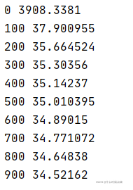
边栏推荐
- What role does 5g era server play in this?
- 103.53.124. What is the difference between X IP BGP line and ordinary dedicated line
- PyTorch学习日记(三)
- How to download free papers from CNKI
- PyTorch学习笔记(一)
- 高防服务器是如何确认哪些是恶意IP/流量?ip:103.88.32.XXX
- 爬虫基础—多线程和多进程的基本原理
- 爬虫基础—Session和Cookie
- ACK攻击是什么意思?ACK攻击怎么防御
- 103.53.124.X IP段BGP线路和普通的专线有什么区别
猜你喜欢

Xiaodi network security - Notes (4)

Arm server building my world (MC) version 1.18.2 private server tutorial

m基于matlab的DQPSK调制解调技术的仿真

Legendary game setup tutorial

传奇手游怎么开服?需要投资多少?需要那些东西?

Data protection / disk array raid protection IP segment 103.103.188 xxx

Utilisation et différenciation des dictionnaires, des tuples et des listes,

Use of urllib Library

IP103.53.125.xxx IP地址段 详解

m基于simulink的16QAM和2DPSK通信链路仿真,并通过matlab调用simulink模型得到误码率曲线
随机推荐
Xiaodi network security - note encryption coding algorithm (6)
Mapping rule configuration of zuul route
爬虫基础—代理的基本原理
阿里云、腾讯云、华为云、Ucloud(优刻得)、天翼云 的云服务器性能测试和价格对比
Debug wechat one hop under linxu (Fedora 27)
Matlab simulation of cognitive femtocell performance in m3gpp LTE communication network
传奇游戏架设教程
Legendary game setup tutorial
m基于matlab的DQPSK调制解调技术的仿真
Arm server building my world (MC) version 1.18.2 private server tutorial
Review summary of MySQL
[automated testing] - robotframework practice (I) building environment
CDN是什么?使用CDN有什么优势?
linux下执行shell脚本调用sql文件,传输到远程服务器
Poor Xiaofan (simulation)
Solve the problem that the unit test coverage of sonar will be 0
天翼云 杭州 云主机(VPS) 性能评测
Performance evaluation and comparison of Huawei cloud Kunpeng arm ECs and x86 ECS
怎么知道网络是否需要用高防服务器?怎么选择机房也是很重要的一点以及后期业务的稳定性
4.IDEA的安装与使用