当前位置:网站首页>Figure an introduction to the interpretable method of neural network and a code example of gnnexplainer interpreting prediction
Figure an introduction to the interpretable method of neural network and a code example of gnnexplainer interpreting prediction
2022-07-19 10:25:00 【deephub】
The interpretability of deep learning model provides human understandable reasoning for its prediction . If you don't explain the reasons behind the prediction , Deep learning algorithms are like black boxes , For some scenes, it can't be trusted . The reason for not providing predictions will also prevent deep learning algorithms from involving cross domain fairness 、 Used in privacy and security critical applications .
The interpretability of deep learning models helps to increase trust in model predictions , Improve model fairness 、 Privacy and other security challenges are related to the transparency of key decision-making applications , And it can let us know the characteristics of the network , In order to identify and correct the system patterns that the model makes mistakes before deploying it to the real world .
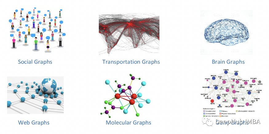
Pictures are everywhere in the real world , On behalf of Social Networks 、 Reference network 、 Chemical molecules 、 Financial data, etc . Figure neural network (GNN) It's a powerful framework , It is used for machine learning of graph related data , For example, node classification 、 Picture classification 、 And link prediction .
So this article discusses the following 5 aspect
- GNN Need to be explicable
- explain GNN The challenge of prediction
- Different GNN Interpreter
- GNNExplainer Visual interpretation of
- Use GNNExplainer Explain the implementation of node classification and graph classification
Convolutional neural network (GCN)、GraphSAGE And figure pay attention to the network (GAT) etc. GNN By recursively passing neural messages along the edges of the input graph , Combine node feature information with graph structure .

Combining graph structure and feature information at the same time will lead to complex models ; therefore , explain GNN The prediction of is challenging .
- Graph data is not as intuitive as image and text , This makes the human understandable interpretation of the graph depth learning model challenging .
- Images and text use grid data ; But in the topology , Information is represented by characteristic matrix and adjacency matrix , Each node has different neighbors . Therefore, the interpretability method of images and texts is not suitable for obtaining high-quality interpretation of graphs .
- Graph node and edge pairs GNN Has made a significant contribution to the final prediction ; therefore GNN The interpretability of requires consideration of these interactions .
- The node classification task predicts the category of nodes by performing message traversal from their neighbors . Information wandering can better understand GNN Reasons for making predictions , But this is more challenging than images and text .
GNN Interpretation method
Graph interpretability requires answering the following questions :
- Which input edges are more critical , Contribute the most to the prediction ?
- Which input nodes are more important ?
- Which node characteristics are more important ?
- What graph pattern will maximize the prediction of a class ?
explain GNN The methods of are divided into two branches according to the type of interpretation they provide . These graph interpretation methods focus on different aspects of graph models , And provide different views to understand GNN Model .
Instance level method : Given an input graph , The case level method interprets the depth model by identifying important input features for prediction .
The model level approach provides general insights and high-level understanding to interpret depth map models . The model level approach focuses on which input graph patterns can lead to GNN Make some kind of prediction .

The above figure shows the explanation GNN In different ways
Instance level methods are distinguished according to the way in which importance scores are obtained , They can be divided into four different branches .
- Gradients/Feature-based Methods gradient or hidden feature graph is used to represent the importance of different input features , The higher the gradient or eigenvalue, the higher the importance . Based on the gradient / The interpretability method of features is widely used in image and text tasks .SA、Guided back propagation、CAM and Grad-CAM Is based on gradient / Examples of interpretable methods of features .
- The disturbance based method monitors the output changes of different input disturbances . When important input information is retained , The forecast should be similar to the original forecast .GNN Different types of masks can be obtained by using different mask generation algorithms to judge the importance of features , Such as GNNExplainer、PGExplainer、ZORRO、GraphMask、Causal Screening and SubgraphX.
- Decomposition method measures the importance of input characteristics by decomposing the original model prediction into several items , These items are regarded as the importance scores of the corresponding input characteristics .
- The proxy method adopts a simple and interpretable proxy model to approximate the prediction of the adjacent region of the input example by the complex depth model . Proxy methods include GraphLime、RelEx and PGM Explainer.
GNNExplainer
GNNExplainer It is a disturbance based method independent of the model , It can be used for any graph based machine learning task based on GNN The prediction of the model provides interpretable reports .
GNNExplainer Learn the soft mask of edge and node characteristics , Then the prediction is explained through the optimization of the mask .
GNNExplainer Will acquire the input graph and identify the compact subgraph structure and a small number of node features that play a key role in prediction .

GNNExplainer Capture important input features by generating masks that convey key semantics , So as to produce a prediction similar to the original prediction . It learns the soft mask of edge and node characteristics , Interpret predictions through mask optimization .
Obtaining masks for input graphs in different ways can obtain important input characteristics . Different masks are also generated according to the type of prediction task , For example, node mask 、 Edge mask and node feature mask .

The generated mask is combined with the input graph , A new graph containing important input information is obtained by element by element multiplication . Last , Enter the new picture into the trained GNN To evaluate the mask and update the mask generation algorithm .
GNNExplainer Example
explain_node() Learn and return a node feature mask and an edge mask , They are explaining GNN It plays an important role in the prediction of node classification .
#Import Library
import numpy as np
import pandas as pd
import os
import torch_geometric.transforms as T
from torch_geometric.datasets import Planetoid
import matplotlib.pyplot as plt
import torch
import torch.nn.functional as F
from torch_geometric.nn import GCNConv, GNNExplainer
import torch_geometric
from torch_geometric.loader import NeighborLoader
from torch_geometric.utils import to_networkx
#Load the Planetoid dataset
dataset = Planetoid(root='.', name="Pubmed")
data = dataset[0]
#Set the device dynamically
device = torch.device('cuda' if torch.cuda.is_available() else 'cpu')
# Create batches with neighbor sampling
train_loader = NeighborLoader(
data,
num_neighbors=[5, 10],
batch_size=16,
input_nodes=data.train_mask,
)
# Define the GCN model
class Net(torch.nn.Module):
def __init__(self):
super().__init__()
self.conv1 = GCNConv(dataset.num_features, 16, normalize=False)
self.conv2 = GCNConv(16, dataset.num_classes, normalize=False)
self.optimizer = torch.optim.Adam(self.parameters(), lr=0.02, weight_decay=5e-4)
def forward(self, x, edge_index):
x = F.relu(self.conv1(x, edge_index))
x = F.dropout(x, training=self.training)
x = self.conv2(x, edge_index)
return F.log_softmax(x, dim=1)
model = Net().to(device)
def accuracy(pred_y, y):
"""Calculate accuracy."""
return ((pred_y == y).sum() / len(y)).item()
# define the function to Train the model
def train_nn(model, x,edge_index,epochs):
criterion = torch.nn.CrossEntropyLoss()
optimizer = model.optimizer
model.train()
for epoch in range(epochs+1):
total_loss = 0
acc = 0
val_loss = 0
val_acc = 0
# Train on batches
for batch in train_loader:
optimizer.zero_grad()
out = model(batch.x, batch.edge_index)
loss = criterion(out[batch.train_mask], batch.y[batch.train_mask])
total_loss += loss
acc += accuracy(out[batch.train_mask].argmax(dim=1),
batch.y[batch.train_mask])
loss.backward()
optimizer.step()
# Validation
val_loss += criterion(out[batch.val_mask], batch.y[batch.val_mask])
val_acc += accuracy(out[batch.val_mask].argmax(dim=1),
batch.y[batch.val_mask])
# Print metrics every 10 epochs
if(epoch % 10 == 0):
print(f'Epoch {epoch:>3} | Train Loss: {total_loss/len(train_loader):.3f} '
f'| Train Acc: {acc/len(train_loader)*100:>6.2f}% | Val Loss: '
f'{val_loss/len(train_loader):.2f} | Val Acc: '
f'{val_acc/len(train_loader)*100:.2f}%')
# define the function to Test the model
def test(model, data):
"""Evaluate the model on test set and print the accuracy score."""
model.eval()
out = model(data.x, data.edge_index)
acc = accuracy(out.argmax(dim=1)[data.test_mask], data.y[data.test_mask])
return acc
# Train the Model
train_nn(model, data.x, data.edge_index, 200)
# Test
print(f'\nGCN test accuracy: {test(model, data)*100:.2f}%\n')
# Explain the GCN for node
node_idx = 20
x, edge_index = data.x, data.edge_index
# Pass the model to explain to GNNExplainer
explainer = GNNExplainer(model, epochs=100,return_type='log_prob')
#returns a node feature mask and an edge mask that play a crucial role to explain the prediction made by the GNN for node 20
node_feat_mask, edge_mask = explainer.explain_node(node_idx, x, edge_index)
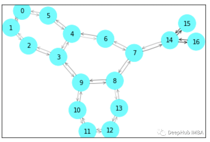
ax, G = explainer.visualize_subgraph(node_idx, edge_index, edge_mask, y=data.y)
plt.show()
print("Ground Truth label for node: ",node_idx, " is ", data.y.numpy()[node_idx])
out = torch.softmax(model(data.x, data.edge_index), dim=1).argmax(dim=1)
print("Prediction for node ",node_idx, "is " ,out[node_idx].cpu().detach().numpy().squeeze())

All nodes with similar colors in the above figure belong to the same class . Visualization helps explain which nodes contribute most to the prediction .
Explain_graph() For graph classification ; It learns and returns a node feature mask and an edge mask , These two masks are explaining GNN It plays a vital role in the prediction of a graph
# Import libararies
import numpy as np
import pandas as pd
import os

import torch_geometric.transforms as T
from torch_geometric.datasets import Planetoid
import matplotlib.pyplot as plt
import torch
import torch.nn.functional as F
from torch_geometric.nn import GraphConv
import torch_geometric
from torch.nn import Parameter
from torch_geometric.nn.conv import MessagePassing
import urllib.request
import tarfile
from torch.nn import Linear
import torch.nn.functional as F
from torch_geometric.nn import GCNConv, GNNExplainer
from torch_geometric.nn import global_mean_pool
from torch_geometric.datasets import TUDataset
from torch_geometric.loader import DataLoader

# Load the dataset
dataset = TUDataset(root='data/TUDataset', name='MUTAG')

# print details about the graph
print(f'Dataset: {dataset}:')
print("Number of Graphs: ",len(dataset))
print("Number of Freatures: ", dataset.num_features)
print("Number of Classes: ", dataset.num_classes)

data= dataset[0]
print(data)
print("No. of nodes: ", data.num_nodes)
print("No. of Edges: ", data.num_edges)
print(f'Average node degree: {data.num_edges / data.num_nodes:.2f}')
print(f'Has isolated nodes: {data.has_isolated_nodes()}')
print(f'Has self-loops: {data.has_self_loops()}')
print(f'Is undirected: {data.is_undirected()}')

# Create train and test dataset
torch.manual_seed(12345)
dataset = dataset.shuffle()

train_dataset = dataset[:50]
test_dataset = dataset[50:]

print(f'Number of training graphs: {len(train_dataset)}')
print(f'Number of test graphs: {len(test_dataset)}')

'''graphs in graph classification datasets are usually small,
a good idea is to batch the graphs before inputting
them into a Graph Neural Network to guarantee full GPU utilization__
_In pytorch Geometric adjacency matrices are stacked in a diagonal fashion
(creating a giant graph that holds multiple isolated subgraphs), a
nd node and target features are simply concatenated in the node dimension:
'''

train_loader = DataLoader(train_dataset,  batch_size=64, shuffle= True)
test_loader= DataLoader(test_dataset,  batch_size=64, shuffle= False)

for step, data in enumerate(train_loader):
    print(f'Step {step + 1}:')
    print('=======')
    print(f'Number of graphs in the current batch: {data.num_graphs}')
    print(data)
    print()

# Build the model
class GNN(torch.nn.Module):
    def __init__(self, hidden_channels):
        super(GNN, self).__init__()
        torch.manual_seed(12345)
        self.conv1 = GraphConv(dataset.num_node_features, hidden_channels)
        self.conv2 = GraphConv(hidden_channels, hidden_channels)

        self.conv3 = GraphConv(hidden_channels, hidden_channels )
        self.lin = Linear(hidden_channels, dataset.num_classes)

    def forward(self, x, edge_index, batch):
        x = self.conv1(x, edge_index)
        x = x.relu()
        x = self.conv2(x, edge_index)
        x = x.relu()
        x = self.conv3(x, edge_index)

        x = global_mean_pool(x, batch)

        x = F.dropout(x, p=0.5, training=self.training)
        x = self.lin(x)

        return x
model = GNN(hidden_channels=64)
print(model)

# set the optimizer
optimizer = torch.optim.Adam(model.parameters(), lr=0.02)

# set the loss function
criterion = torch.nn.CrossEntropyLoss()

# Creating the function to train the model
def train():
    model.train()

    for data in train_loader:  # Iterate in batches over the training dataset.
         out = model(data.x, data.edge_index, data.batch)  # Perform a single forward pass.
         loss = criterion(out, data.y)  # Compute the loss.
         loss.backward()  # Derive gradients.
         optimizer.step()  # Update parameters based on gradients.
         optimizer.zero_grad()  # Clear gradients.

# function to test the model
def test(loader):
     model.eval()

     correct = 0
     for data in loader:  # Iterate in batches over the training/test dataset.
         out = model(data.x, data.edge_index, data.batch)
         pred = out.argmax(dim=1)  # Use the class with highest probability.
         correct += int((pred == data.y).sum())  # Check against ground-truth labels.
     return correct / len(loader.dataset)  # Derive ratio of correct predictions.

# Train the model for 150 epochs
for epoch in range(1, 160):
    train()
    train_acc = test(train_loader)
    test_acc = test(test_loader)
    if(epoch % 10 == 0):
          '''print(f'Epoch {epoch:>3} | Train Loss: {total_loss/len(train_loader):.3f} '
                f'| Train Acc: {acc/len(train_loader)*100:>6.2f}% | Val Loss: '
                f'{val_loss/len(train_loader):.2f} | Val Acc: '
                f'{val_acc/len(train_loader)*100:.2f}%')
          '''
          print(f'Epoch: {epoch:03d}, Train Acc: {train_acc:.4f}, Test Acc: {test_acc:.4f}')

#Explain the Graph
explainer = GNNExplainer(model, epochs=100,return_type='log_prob')
data = dataset[0]
node_feat_mask, edge_mask = explainer.explain_graph(data.x, data.edge_index)
ax, G = explainer.visualize_subgraph(-1,data.edge_index, edge_mask, data.y)
plt.show()
When visualizing visualize_subgraph when , Need to put node_idx Set to -1, Because this means a graph classification task ; Otherwise, an error will be reported .
This article USES pytorch-geometric Realized GNNExplainer As an example , If you are interested, you can check its official documents
https://avoid.overfit.cn/post/3a01457fe6094941a2bca2961f742dce
author :Renu Khandelwal
边栏推荐
猜你喜欢


随机推荐
Microsoft OneNote 教程,如何在 OneNote 中插入数学公式?
Ffmpeg merges multiple videos (vb.net, class library-8)
HCIA OSPF
HCIA rip experiment 7.11
Simulation Research on optimal detection of fault data in communication network
FFmpeg录制视频、停止(VB.net,踩坑,类库——10)
NJCTF 2017messager
智能存储柜控制系统设计及仿真
Blender自动化建模入门
yarn(cdh)中的虚拟cpu和内存
2022年湖南省中职组“网络空间安全”数据包分析infiltration.pacpng解析(超详细)
STM32F407 NVIC
王者荣耀商城异地多活架构设计
2022年湖南 省中职组“网络空间安全”Windows渗透测试 (超详细)
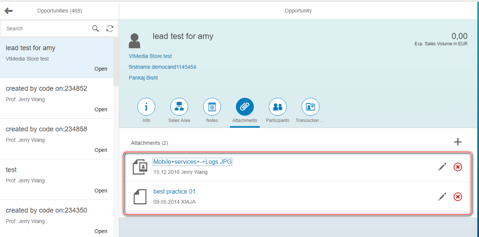
SAP Fiori 的附件处理(Attachment handling)
Huawei wireless device configuration intelligent roaming
HCIP 第一天 7.15
C语言自定义类型详解
HCIA static comprehensive experiment report 7.10
2022 Zhejiang secondary vocational group "Cyberspace Security" code information acquisition and analysis (full version)