[1] The overview

  6 The basic evaluation indicators are as follows: mind map ：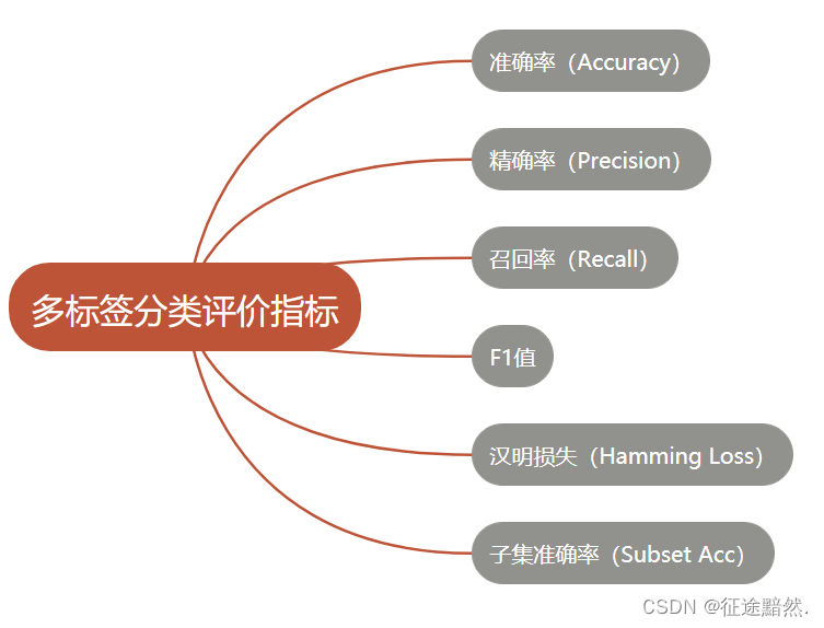

[2] Introduce

   Suppose there's data ： Sample size batch_size = 5, Number of tags label_num = 4.y_true For real labels ,y_pred Is the predicted tag value .

y_true = np.array([[0, 1, 0, 1],
                   [0, 1, 1, 0],
                   [0, 0, 1, 0],
                   [1, 1, 1, 0],
                   [1, 0, 1, 1]])

y_pred = np.array([[0, 1, 1, 0],
                   [0, 1, 1, 0],
                   [0, 0, 1, 0],
                   [0, 1, 1, 0],
                   [0, 1, 0, 1]])

[2.1] Subset accuracy （Subset Accuracy）

   For every sample , The prediction is correct only when the predicted value is exactly the same as the real value , That is to say, as long as there is a difference in the prediction results of one category, it is considered that the prediction is not correct . therefore , Its calculation formula is ：

   Compare the data given above y_true、y_pred. Then only the second 2 And the first 3 It's a sample that makes the prediction right . stay sklearn in , You can go directly through sklearn.metrics Module accuracy_score Method to complete the calculation [3], Code implementation ：

from sklearn.metrics import accuracy_score

print(accuracy_score(y_true,y_pred)) # 0.4

print(accuracy_score(y_true,y_pred,normalize=False)) # 2

【 notes 】
accuracy_score With parameters normalize.
normalize = False when ： Return the exact number of samples ,
normalize = True when ： Return the proportion of completely correct samples .

[2.2] Accuracy rate （Accuracy）

   Accuracy is the average accuracy of all samples . And for each sample , The accuracy rate is the proportion of the number of correctly predicted tags in the total number of correctly predicted or actually correct tags . Its calculation formula is ：

   For example, for a sample , Its real label is [0, 1, 0, 1], The prediction label is [0, 1, 1, 0]. Then the corresponding accuracy of the sample should be ：（0 + 1 + 0 + 0） / （0 + 1 + 1 + 1）= 0.33.

   Compare the data given above y_true、y_pred. Then the corresponding accuracy of the sample should be ：
$$\frac{1}{5}\ast (\frac{1}{3}+\frac{2}{2}+\frac{1}{1}+\frac{2}{3}+\frac{1}{4})=0.65$$

   stay sklearn in ,acc Subset accuracy only , So here we need to realize by ourselves . Code implementation ：

def Accuracy(y_true, y_pred):
    count = 0
    for i in range(y_true.shape[0]):
        p = sum(np.logical_and(y_true[i], y_pred[i]))
        q = sum(np.logical_or(y_true[i], y_pred[i]))
        count += p / q
    return count / y_true.shape[0]
    
print(Accuracy(y_true, y_pred)) # 0.65

[2.3] Accuracy （Precision）

   The accuracy rate calculates the average accuracy rate of all samples . And for each sample , The accuracy rate is the proportion of the number of correctly predicted tags in the total number of correctly predicted tags . Its calculation formula is ：

   For example, for a sample , Its real label is [0, 1, 0, 1], The prediction label is [0, 1, 1, 0]. Then the accuracy of the sample should be ：（0 + 1 + 0 + 0） / （1 + 1）= 0.5.

   Compare the data given above y_true、y_pred. Then the corresponding accuracy of the sample should be ：
$$\frac{1}{5}\ast (\frac{1}{2}+\frac{2}{2}+\frac{1}{1}+\frac{2}{2}+\frac{1}{2})=0.8$$

   Code implementation ：

from sklearn.metrics import precision_score

print(precision_score(y_true=y_true, y_pred=y_pred, average='samples'))# 0.8

[2.4] Recall rate （Recall）

   Recall rate is actually the average recall rate of all samples . And for each sample , Recall rate is to predict the proportion of the correct number of tags in the total number of correct tags . Its calculation formula is ：

   For example, for a sample , Its real label is [0, 1, 0, 1], The prediction label is [0, 1, 1, 0]. Then the accuracy of the sample should be ：（0 + 1 + 0 + 0） / （1 + 1）= 0.5.

   Compare the data given above y_true、y_pred. Then the corresponding accuracy of the sample should be ：
$$\frac{1}{5}\ast (\frac{1}{2}+\frac{2}{2}+\frac{1}{1}+\frac{2}{3}+\frac{1}{3})=0.7$$

   Code implementation ：

from sklearn.metrics import recall_score

print(recall_score(y_true=y_true, y_pred=y_pred, average='samples'))# 0.7

[2.5] F1

   Its calculation formula is ：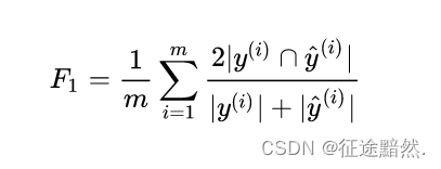

   For example, for a sample , Its real label is [0, 1, 0, 1], The prediction label is [0, 1, 1, 0]. Then the accuracy of the sample should be ：2 * （0 + 1 + 0 + 0） / （（1 + 1）+（1 + 1））= 0.5.

   Compare the data given above y_true、y_pred. Then the corresponding accuracy of the sample should be ：
$$2\ast \frac{1}{5}\ast (\frac{1}{4}+\frac{2}{4}+\frac{1}{2}+\frac{2}{5}+\frac{1}{5})=0.74$$

   Code implementation ：

from sklearn.metrics import f1_score

print(f1_score(y_true,y_pred,average='samples'))# 0.74

[2.6] Hamming lost （Hamming Loss）

  Hamming Loss It's measured in all samples , The proportion of mispredicted tags in the total number of tags . So for Hamming Loss In terms of losses , The smaller the value, the better the performance of the model .
   Compare the data given above y_true、y_pred. Then the corresponding accuracy of the sample should be ：
$$\frac{1}{5\ast 4}\ast (2+0+0+1+3)=0.3$$

   Code implementation ：

from sklearn.metrics import hamming_loss
print(hamming_loss(y_true, y_pred))# 0.3