当前位置:网站首页>Study notes of automatic control principle -- correction and synthesis of automatic control system
Study notes of automatic control principle -- correction and synthesis of automatic control system
2022-07-26 08:54:00 【Miracle Fan】
Self control principle learning notes
Self control principle learning notes column
Chapter one —— Dynamic model of feedback control system
Chapter two —— Stability analysis of control system
The third chapter —— Continuous time system performance analysis
Chapter four —— Calibration and synthesis of automatic control system
The fifth chapter —— Linear discrete system
Calibration and synthesis of automatic control system
List of articles
1. Basic concepts of control system synthesis and correction
1.1 Comprehensive introduction to the system
Give a certain design index in advance , This indicator is usually given in strict mathematical form , Then determine some control form or index based on the structure to get the desired system , Then find the controller that meets the predetermined index through analysis .
Is to seek the right number of tools and put forward the right indicators .
1.2 System calibration
Develop the expected performance indicators of the system , Based on these performance indicators and uncorrected system characteristics , Determine the structure of the correction , Through the comparison and calculation of indicators, the control parameters in the correction structure are determined .
The initial state of the time response corresponds to the high frequency characteristics of the frequency response , The final state of the time response corresponds to the low-frequency characteristics of the frequency response , The transient of the time response corresponds to the crossover region of the frequency response .
1.3 Rough correspondence between time response and frequency characteristics
The initial state of the time response corresponds to the high frequency characteristics of the frequency response , The final state of the time response corresponds to the low-frequency characteristics of the frequency response , The transient of the time response corresponds to the crossover region of the frequency response .
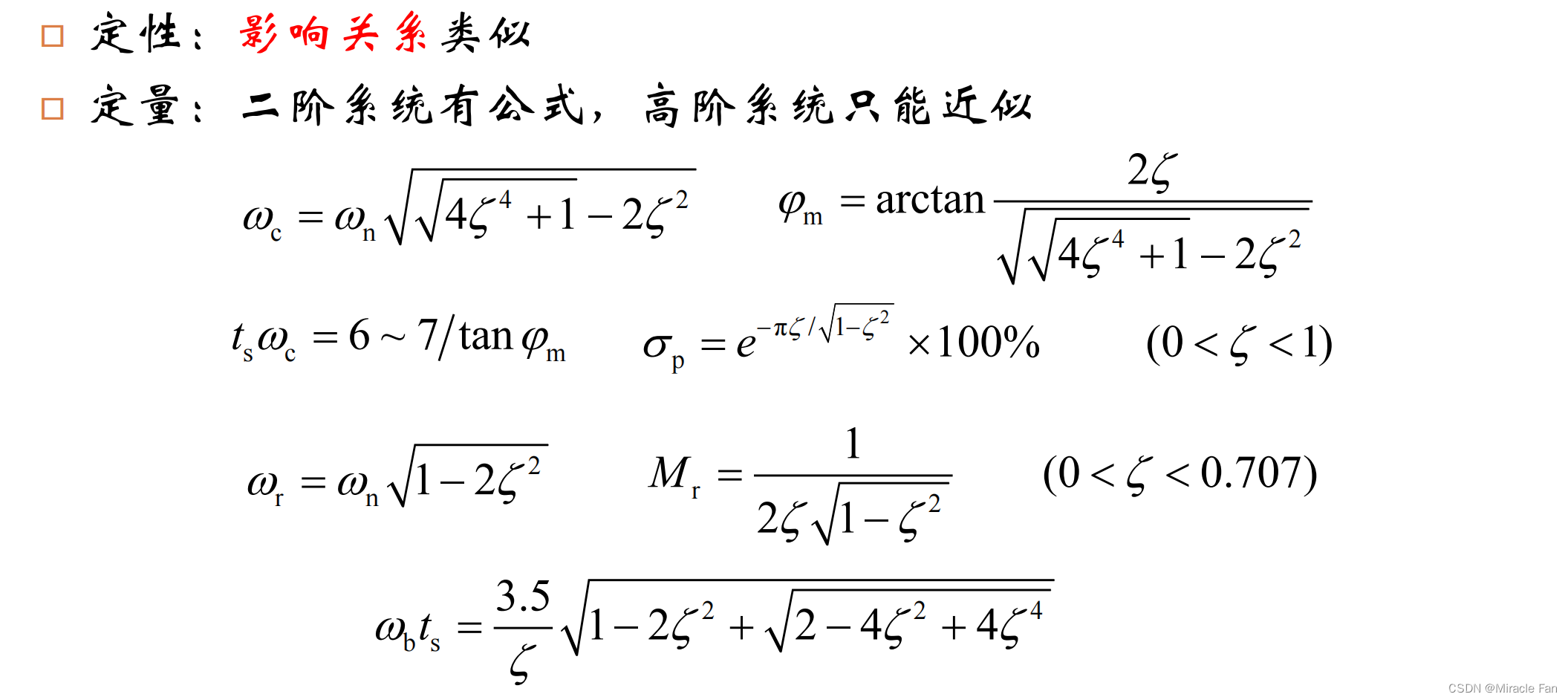
1.4 Index type
Performance indicators mainly include time domain indicators and frequency domain indicators , It is generally difficult to accurately establish the relationship between the two , At a glance , The initial state of the time response corresponds to the high frequency characteristics of the frequency response , The last state of the time response corresponds to the low-frequency characteristics of the frequency response , The transient of time response corresponds to the intermediate frequency characteristics of frequency response .
1. Static indicators : Steady state error
2. Time domain dynamic index : Adjust the time 、 Peak time 、 Overshoot
3. Frequency domain dynamic index :
Open loop : Crossover frequency 、 Phase margin
closed loop : Resonant frequency 、 Resonance peak 、 Bandwidth frequency
1.5 Relationship between dynamic performance indicators
2. Loop shaping
The idea of loop shaping :
Closed loop performance index -> Desired open-loop frequency characteristics -> controller
2.1 Controller output requirements
Low frequency band : Open loop gain K K K, System type v → v\rightarrow v→ Steady state error e s s e_{ss} ess, Hope the shape is steep , high
If band : Cut off frequency w c w_c wc, Phase margin γ \gamma γ, Dynamic performance : σ % , t s \sigma\%,t_s σ%,ts, Hope the shape is slow , wide
High frequency band : The ability of the system to resist high-frequency interference , High frequency roll off characteristics are expected , Hope the shape is low , steep
3. Series correction
3.1 Series lead correction
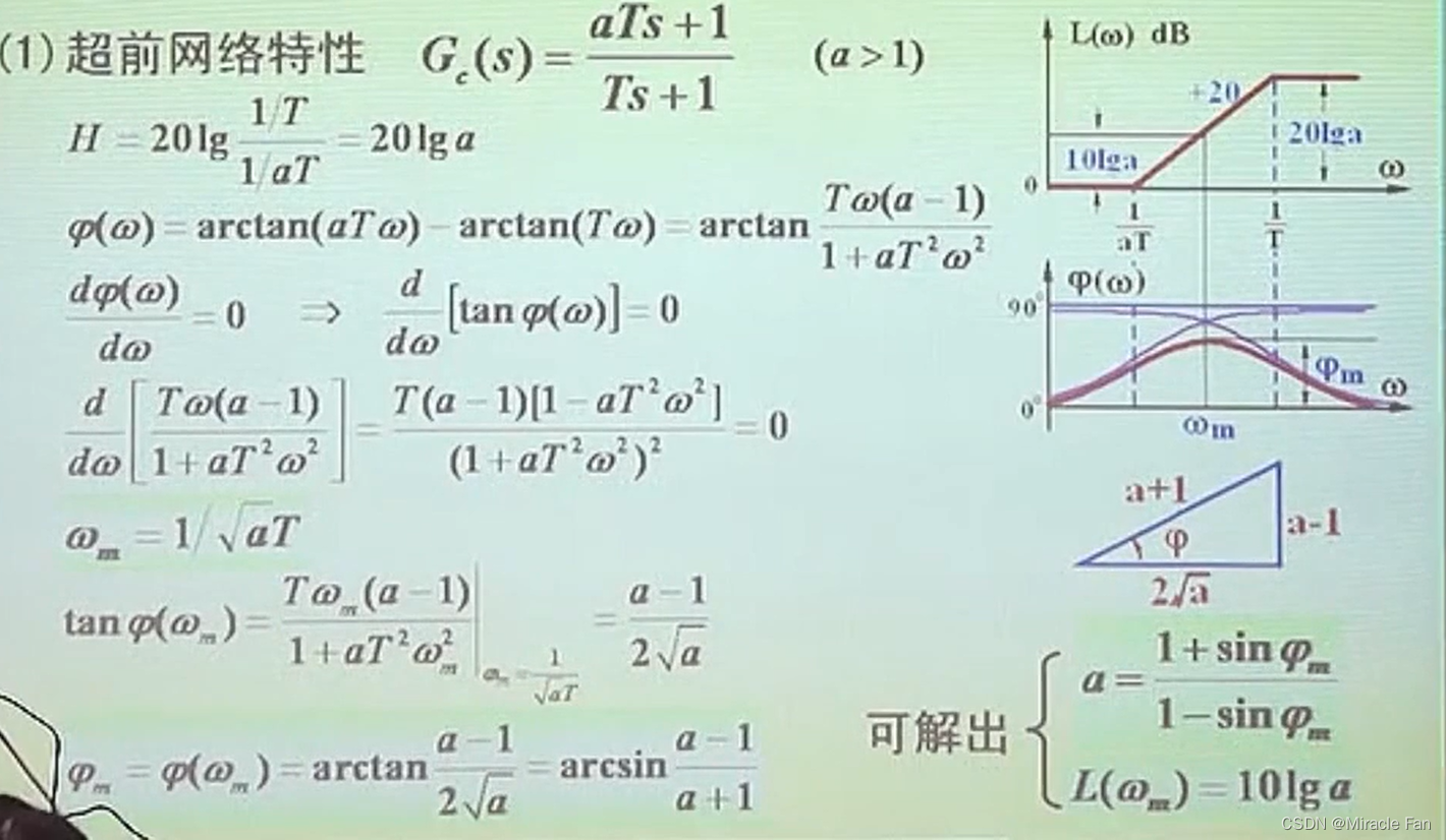
G c ( s ) = a T s + 1 T s + 1 ( a > 1 ) G_c(s)=\frac{aTs+1}{Ts+1}(a>1) Gc(s)=Ts+1aTs+1(a>1)
a Usually take 4~10, The maximum lead angle of the primary lead network is 60 degree , The phase angle is ahead , The amplitude increases
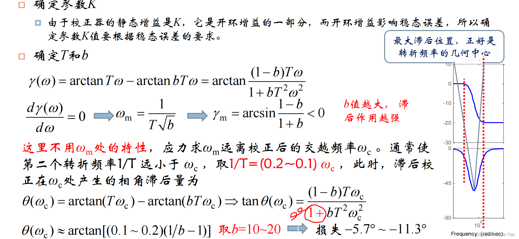
The essence : Using the phase angle advance characteristic of the lead network to improve the phase angle margin of the system , Put the controller Frequency at the maximum lead angle Just controlled in Crossing frequency It's about , In this way, the improved phase margin is the best .
Advance correction steps ( e s s ∗ , w c ∗ , γ ∗ ) (e_{ss}^*,w_c^*,\gamma^*) (ess∗,wc∗,γ∗): An asterisk indicates the index requirements
- Through the given steady-state error e s s ∗ = s R ( s ) 1 + L ( S ) e_{s s}^{*}=\frac{sR(s)}{1+L(S)} ess∗=1+L(S)sR(s) To calculate the K value
- adopt K P ( i w ) KP(iw) KP(iw), Calculate the crossing frequency at this time w c 0 , γ 0 w_{c0},\gamma_0 wc0,γ0, Judge , Such as w c 0 , γ 0 w_{c0},\gamma_0 wc0,γ0 Is it not enough The fruit is not enough , Then advance correction can be adopted
- Calculation C ( s ) C(s) C(s) The maximum lead angle to be provided φ m = γ ∗ − γ 0 + ( 5 ∘ ∼ 1 0 ∘ ) \varphi_{m}=\gamma^{*}-\gamma_{0}+\left(5^{\circ} \sim 10^{\circ}\right) φm=γ∗−γ0+(5∘∼10∘),
( 5 ∘ ∼ 1 0 ∘ ) \left(5^{\circ} \sim 10^{\circ}\right) (5∘∼10∘) Used to compensate for the increase of crossing frequency , Cause the original P ( s ) P(s) P(s) The loss of phase angle reduction provided at the corresponding crossing frequency . here a According to the formula a = 1 + sin φ m 1 − sin φ m a=\frac{1+\sin \varphi_{m}}{1-\sin \varphi_{m}} a=1−sinφm1+sinφm To calculate the . meanwhile C ( s ) C(s) C(s) The amplitude frequency characteristic provided at the maximum lead angle is 10 lg a 10\lg {a} 10lga. - take ∣ K P ( i w c ) ∣ = − 10 lg a |KP(iw_c)|=-10\lg a ∣KP(iwc)∣=−10lga, That is to say C ( s ) C(s) C(s) Frequency at the maximum lead angle , Calculate the corrected crossing frequency w c w_c wc, And then through the formula τ = 1 a w c \tau = \frac{1}{\sqrt{a}w_c} τ=awc1 To calculate the τ \tau τ.
- take C ( s ) C(s) C(s) Plug in P ( s ) P(s) P(s) Calculate whether the phase margin and crossing frequency of the corrected system meet the requirements
effect :
- Keep the low band : Meet the steady-state accuracy e s s e_{ss} ess
- Improve the intermediate frequency band : w c ↑ , γ 0 ↑ w_c \uparrow,\gamma_0 \uparrow wc↑,γ0↑, Improved dynamic performance , The signal reproduction ability is improved , Improve the rapidity of the system
- Raise the high band : The ability to resist high-frequency interference decreases , Raise the amplitude frequency characteristic .
3.2 PD correction
wave filtering PD correction :
C ( s ) = K p ( 1 + T d s T d s / N + 1 ) C(s)=K_p(1+\frac{T_ds}{T_ds/N+1}) C(s)=Kp(1+Tds/N+1Tds)
Compared with the ideal PD Adjust the , wave filtering PD Regulation is an additional inertia link in its controller .
In time K p = K , T d = a τ , T d / N = τ , N = a K_p=K,T_d=a\tau,T_d/N=\tau,N=a Kp=K,Td=aτ,Td/N=τ,N=a, So it can be solved by the series advance correction algorithm .
No filtering PD correction ( Ideal filtering PD):
C ( s ) = K p ( 1 + T d s ) C(s)=K_p(1+T_ds) C(s)=Kp(1+Tds)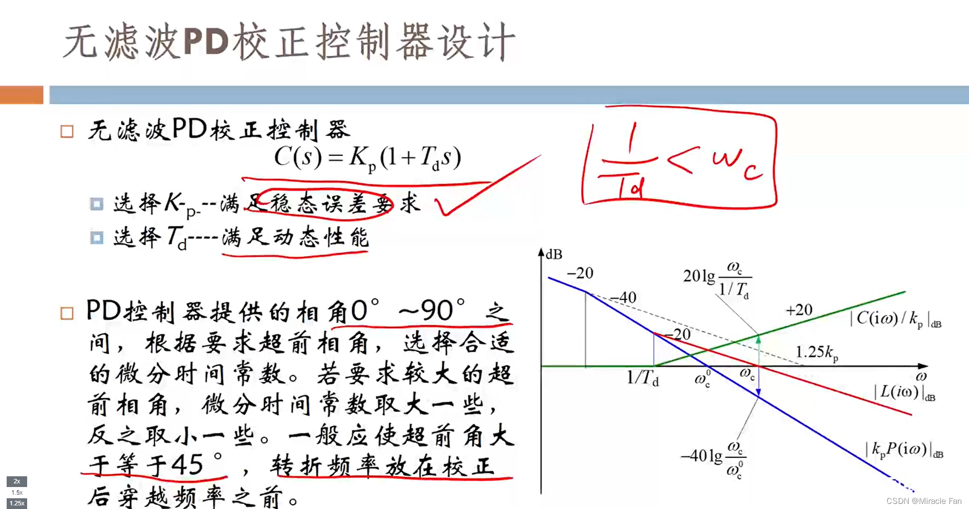
3.2 Series lag correction
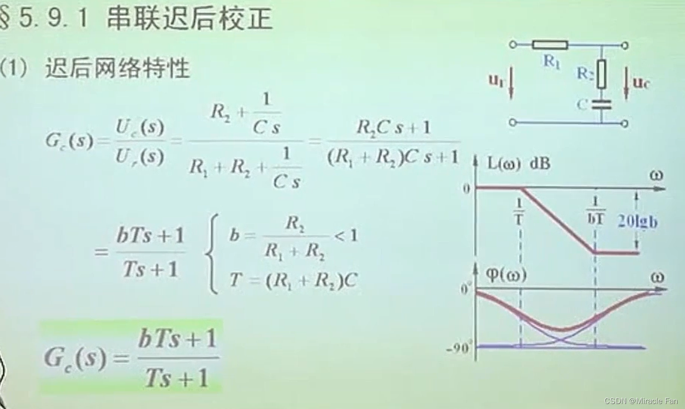
G c ( s ) = b T s + 1 T s + 1 ( b < 1 ) G_c(s)=\frac{bTs+1}{Ts+1}(b<1) Gc(s)=Ts+1bTs+1(b<1)
The essence : Using the high-frequency amplitude attenuation characteristics of the lag correction device , Reduce the transient gain and ride through frequency of the system , Excavate the reserves of the phase angle of the system itself
Lag correction steps :
According to the given steady-state error requirements , Calculate the static gain of the controller K
adopt K P ( i w ) KP(iw) KP(iw) Of Bode chart , Calculate the crossover frequency and phase margin , When the crossing frequency is enough , When the phase margin is insufficient, the lag correction is generally used .
According to the phase margin , Determine the crossover frequency of the system after correction w c ∗ w_c^* wc∗
18 0 ∘ + ∠ K P ( i ω c ∗ ) ≥ φ m ∗ + δ , δ = 5 ∼ 2 0 ∘ 180^{\circ}+\angle K P\left(\mathrm{i} \omega{ }_{\mathrm{c}}^{*}\right) \geq \varphi_{\mathrm{m}}^{*}+\delta, \quad \delta=5 \sim 20^{\circ} 180∘+∠KP(iωc∗)≥φm∗+δ,δ=5∼20∘
Because for lag correction , We are mainly Excavate the phase angle reserve of the original system , Not through the maximum hysteresis angle of the controller , And the crossing frequency should be far away from the frequency corresponding to the maximum hysteresis angle , So here The phase angle provided by the controller is omitted .Find out K P ( i w ) KP(iw) KP(iw) At the new crossing frequency dB value , This value is offset with the medium and high frequency band of the controller . That is to say
20 lg b = ∣ K P ( i w c ∗ ) ∣ 20\lg b = |KP(iw_c^*)| 20lgb=∣KP(iwc∗)∣Then pass the order T = ( 1 5 ∼ 1 10 ) w c ∗ T=(\frac{1}{5} \sim \frac{1}{10})w_c^* T=(51∼101)wc∗
Determine the correction device , And further verify .
effect :
- Keep the low band : Meet the steady-state accuracy e s s e_{ss} ess
- Lower the intermediate frequency band : w c ↓ , γ ↑ w_c \downarrow,\gamma \uparrow \quad wc↓,γ↑ Lose quickness , Improve uniformity
- Lower the high frequency band : The ability to resist high-frequency interference is improved
3.3 PI correction
ratio K p K_p Kp No longer based on the steady-state error requirements of the system , It is used to offset the amplitude of the pull down .
C ( s ) = k p ( 1 + 1 T i s ) C(s)=k_p(1+\frac{1}{T_is}) C(s)=kp(1+Tis1)
3.4 Lag lead correction
The essence : Comprehensive utilization of lagging network attenuation , The phase angle of lead network is advanced , Transform the open-loop characteristic and frequency characteristic , Improve system performance
Calibration steps :
- Select the gain of the controller K c K_c Kc, Use the given steady-state error requirements
- K P ( i w ) KP(iw) KP(iw) Of Bode chart , Determine whether lag lead correction is required
- Select the lower limit of the expected crossing frequency , Determine the maximum lead angle that needs to be provided , Similar to the solution of lead correction
- Introduce lag correction , bring K P C 1 {\color{red}KPC_1} KPC1 stay w c w_c wc The amplitude at is 1, Calculate the relevant parameters of lag correction

Be careful :b<a The parameter setting of is not conducive to suppressing high-frequency noise .
3.5PID correction
Similar to the previous PD and PI correction , Note that this time K p K_p Kp effect Consistent with standard lag lead correction , Although the design methods are different .
边栏推荐
- SSH,NFS,FTP
- Day06 operation -- addition, deletion, modification and query
- day06 作业--技能题6
- Oracle 19C OCP 1z0-083 question bank (7-12)
- uni-app 简易商城制作
- Learning notes of automatic control principle --- linear discrete system
- node的js文件引入
- Oracle 19C OCP certification examination software list
- Neo eco technology monthly | help developers play smart contracts
- Excel find duplicate lines
猜你喜欢


随机推荐
6、 Pinda general permission system__ pd-tools-log
[recommended collection] MySQL 30000 word essence summary + 100 interview questions (I)
ES6模块化导入导出)(实现页面嵌套)
OA项目之我的会议(会议排座&送审)
CIS 2020 - alternative skills against cloud WAF (pyn3rd)
Xshell batch send command to multiple sessions
Oracle 19C OCP 1z0-082 certification examination question bank (19-23)
解决C#跨线程调用窗体控件的问题
Analysis on the query method and efficiency of Oracle about date type
Cve-2021-21975 VMware SSRF vulnerability recurrence
[freeswitch development practice] use SIP client Yate to connect freeswitch for VoIP calls
Oracle 19C OCP 1z0-082 certification examination question bank (24-29)
The lessons of 2000. Web3 = the third industrial revolution?
Day06 homework -- skill question 2
海内外媒体宣发自媒体发稿要严格把握内容关
Use index to optimize SQL query "suggestions collection"
C Entry series (31) -- operator overloading
2000年的教训。web3是否=第三次工业革命?
One click deployment of lamp and LNMP scripts is worth having
My meeting of OA project (meeting seating & submission for approval)