当前位置:网站首页>Wu Enda's machine learning after class exercises - linear regression
Wu Enda's machine learning after class exercises - linear regression
2022-07-26 04:15:00 【Yizhou YZ】
Univariate linear regression
import numpy as np
import pandas as pd
import matplotlib.pyplot as plt
path = "ex1data1.txt"
data = pd.read_csv(path, header=None, names=['Population', 'Profit'])
# pandas.read_csv By default, the first row of the data content will be defaulted to the field name Title ,header=None Indicates that the read raw file data has no column index
data.head() #  Method is used to return the first... Of a data frame or sequence n That's ok ( The default value is 5). Return type :DataFrame, It can be understood as a table , Or matrix
# DataFrame It is essentially a two-dimensional matrix , The difference from the conventional two-dimensional matrix is that the former additionally specifies the names of each row and column .
| Population | Profit | |
|---|---|---|
| 0 | 6.1101 | 17.5920 |
| 1 | 5.5277 | 9.1302 |
| 2 | 8.5186 | 13.6620 |
| 3 | 7.0032 | 11.8540 |
| 4 | 5.8598 | 6.8233 |
data.describe()
# describe()  Function can view the basic situation of data ,
#  Include :count  Non null number 、mean  Average 、std  Standard deviation 、max  Maximum 、min  minimum value 、(25%、50%、75%) Quantiles, etc. .
| Population | Profit | |
|---|---|---|
| count | 97.000000 | 97.000000 |
| mean | 8.159800 | 5.839135 |
| std | 3.869884 | 5.510262 |
| min | 5.026900 | -2.680700 |
| 25% | 5.707700 | 1.986900 |
| 50% | 6.589400 | 4.562300 |
| 75% | 8.578100 | 7.046700 |
| max | 22.203000 | 24.147000 |
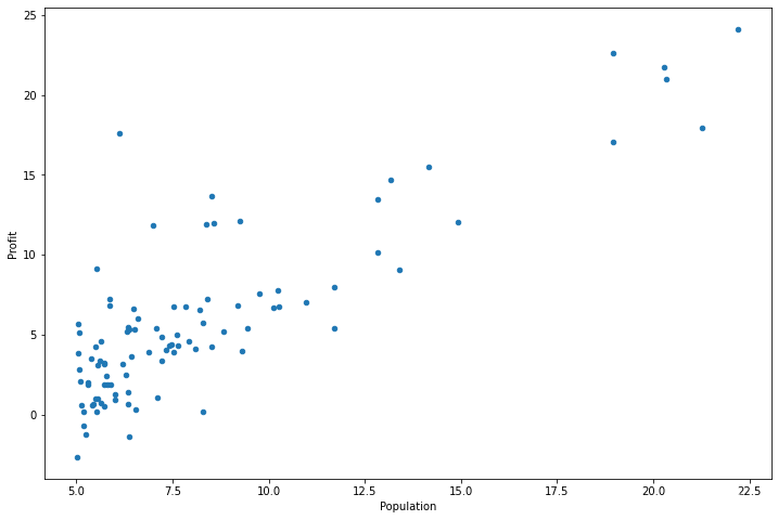
#  Draw a picture
data.plot(kind='scatter',x='Population',y='Profit',figsize=(12,8))
# scatter Represents a scatter plot ,figsize Show the size of the picture , Company : Inch
plt.show()
Use gradient descent to minimize the cost function ,
Create a parameter to θ Is the cost function of the characteristic function
J ( θ ) = 1 2 m ∑ i = 1 m ( h θ ( x ( i ) ) − y ( i ) ) 2 J\left( \theta \right)=\frac{1}{2m}\sum\limits_{i=1}^{m}{ { {\left( { {h}_{\theta }}\left( { {x}^{(i)}} \right)-{ {y}^{(i)}} \right)}^{2}}} J(θ)=2m1i=1∑m(hθ(x(i))−y(i))2
among :
h θ ( x ) = θ T X = θ 0 x 0 + θ 1 x 1 + θ 2 x 2 + . . . + θ n x n { {h}_{\theta }}\left( x \right)={ {\theta }^{T}}X={ {\theta }_{0}}{ {x}_{0}}+{ {\theta }_{1}}{ {x}_{1}}+{ {\theta }_{2}}{ {x}_{2}}+...+{ {\theta }_{n}}{ {x}_{n}}\\ hθ(x)=θTX=θ0x0+θ1x1+θ2x2+...+θnxn
def computeCost(X,y,theta): #  Input X Is a column vector ,y It's also a column vector ,theta It's a line vector
    inner = np.power(((X*theta.T)-y),2) # x*θ The transpose of is a hypothetical function  power Function calculation numpy The specified power of each value in the array
    return np.sum(inner/(2*len(X))) #  Will array / All the elements in the matrix add up  len(X) Number of matrix lines
data.insert(0,'Ones',1)
#  Insert a column as 1 For better vectorization , You need to add a column to the training set x_0, So that we can use the vectorized solution to calculate the cost and gradient , See video p18
#  Initialization of a variable
cols = data.shape[1] # shape[0] It's the number of lines  shape[1] It's the number of columns
X = data.iloc[:,0:cols-1] #  Data sets   All right   List from 0 To cols-1( barring )  Left closed right away
y = data.iloc[:,cols-1:cols] #  The target
X.head()
| Ones | Population | |
|---|---|---|
| 0 | 1 | 6.1101 |
| 1 | 1 | 5.5277 |
| 2 | 1 | 8.5186 |
| 3 | 1 | 7.0032 |
| 4 | 1 | 5.8598 |
The data type obtained is DataFrame type , So you need to do type conversion . Initialization is also required theta, namely theta All elements are set to 0
X = np.matrix(X.values)
y = np.matrix(y.values)
theta = np.matrix(np.array([0,0]))
dimension
X.shape, theta.shape, y.shape
((97, 2), (1, 2), (97, 1))
computeCost(X,y,theta) # Computational cost function
32.072733877455676
batch gradient decent( Batch gradient descent )
θ j : = θ j − α ∂ ∂ θ j J ( θ ) { {\theta }_{j}}:={ {\theta }_{j}}-\alpha \frac{\partial }{\partial { {\theta }_{j}}}J\left( \theta \right) θj:=θj−α∂θj∂J(θ)
gradient descent
def gradientDescent(X,y,theta,alpha,iters): # iters Is the number of iterations  alpha It's the learning rate   That is, step length
    temp_theta = np.matrix(np.zeros(theta.shape)) #  Zero value matrix   The staging theta
    parameters = int(theta.ravel().shape[1]) # ravel Calculate the number of parameters to be solved   Function reduces multidimensional array to one dimension   The value here is 2
    cost = np.zeros(iters) # structure iters individual 0 Array of
    # iteration :
    for i in range(iters):
        difference = (X*theta.T) - y #  Difference value
        for j in range(parameters):
            term = np.multiply(difference,X[:,j])    # multiply x_i X[:,j] Represents all lines  j Column , In short, draw out the number j Column
             #  Note that this is not matrix multiplication   Here is the multiplication after derivation  multiply Is the number of corresponding positions of two matrices of the same size multiplied directly
            temp_theta[0,j] = theta[0,j] - (alpha/len(X))*np.sum(term) #  to update theta_j

        theta = temp_theta #  Update all theta value
        cost[i] = computeCost(X,y,theta) #  Renewal value

    return theta,cost
Initialize some additional variables - Learning rate α And the number of iterations to perform .
alpha = 0.01
iters = 1000
obtain theta value , Minimum cost
g,cost = gradientDescent(X,y,theta,alpha,iters)
g
matrix([[-3.24140214, 1.1272942 ]])
cost[-1] # Get the last value of the array
4.515955503078913
Last , Use what we fitted theta Value calculation of the cost function of the training model
computeCost(X, y, g)
4.515955503078913
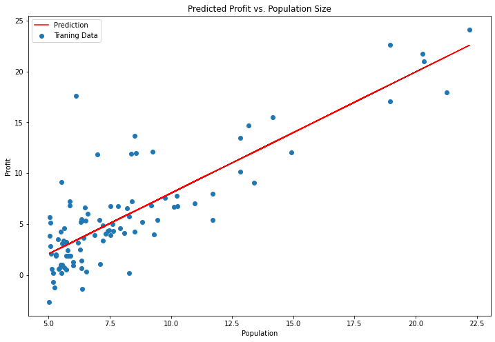
Draw linear models and data , Intuitively see its fitting
x = np.linspace(data.Population.min(), data.Population.max(), 100) #  Generates a one-dimensional array of the specified number within the specified range
f = g[0, 0] + (g[0, 1] * x) # x1=1 g[0, 0] Express theta_0 g[0, 1] Express theta_1

fig, ax = plt.subplots(figsize=(12,8)) # plt.subplot() Function is used to directly specify the division method and position for drawing .
# fig Represents the drawing window (Figure);ax Represents the coordinate system on this drawing window (axis), Will generally continue to ax To operate .

#  Function to set the abscissa and ordinate , And set the color to red , Mark... On the icon 'Prediction' label   Abscissa x  Ordinate f
ax.plot(x, f, 'r', label='Prediction')
#  Define the abscissa and ordinate of the scatter chart , The of scatter plot points is given 'Traning Data' Tag name
ax.scatter(data.Population, data.Profit, label='Traning Data')
ax.legend(loc=2)  # 2 In the upper left corner


ax.set_xlabel('Population')
ax.set_ylabel('Profit')
ax.set_title('Predicted Profit vs. Population Size')
plt.show()

Since the gradient equation function also outputs a cost vector in each training iteration , So we can also draw . Be careful , The cost is always lower
fig, ax = plt.subplots(figsize=(12,8))
ax.plot(np.arange(iters), cost, 'r')
ax.set_xlabel('Iterations')
ax.set_ylabel('Cost')
ax.set_title('Error vs. Training Epoch')
plt.show()

Multivariate linear regression
This exercise includes a housing price data set , It contains two variables ( The size of the house 、 Number of bedrooms ) And the target ( House price ).
path =  'ex1data2.txt'
data2 = pd.read_csv(path, header=None, names=['Size', 'Bedrooms', 'Price'])
data2.head()
| Size | Bedrooms | Price | |
|---|---|---|---|
| 0 | 2104 | 3 | 399900 |
| 1 | 1600 | 3 | 329900 |
| 2 | 2400 | 3 | 369000 |
| 3 | 1416 | 2 | 232000 |
| 4 | 3000 | 4 | 539900 |
data2.describe()
| Size | Bedrooms | Price | |
|---|---|---|---|
| count | 47.000000 | 47.000000 | 47.000000 |
| mean | 2000.680851 | 3.170213 | 340412.659574 |
| std | 794.702354 | 0.760982 | 125039.899586 |
| min | 852.000000 | 1.000000 | 169900.000000 |
| 25% | 1432.000000 | 3.000000 | 249900.000000 |
| 50% | 1888.000000 | 3.000000 | 299900.000000 |
| 75% | 2269.000000 | 4.000000 | 384450.000000 |
| max | 4478.000000 | 5.000000 | 699900.000000 |
The house is about the size of the number of bedrooms 1000 times . When features differ by several orders of magnitude , First perform feature scaling ( Mean normalization ) It can make the gradient descent converge faster .
data2 = (data2 - data2.mean()) / data2.std() #  The solution is to try to scale all feature scales to  -1 ~ 1
data2.head()
| Size | Bedrooms | Price | |
|---|---|---|---|
| 0 | 0.130010 | -0.223675 | 0.475747 |
| 1 | -0.504190 | -0.223675 | -0.084074 |
| 2 | 0.502476 | -0.223675 | 0.228626 |
| 3 | -0.735723 | -1.537767 | -0.867025 |
| 4 | 1.257476 | 1.090417 | 1.595389 |
data2.insert(0, 'Ones', 1)
cols = data2.shape[1]
X2 = data2.iloc[:,0:cols-1]
y2 = data2.iloc[:,cols-1:cols]

X2 = np.matrix(X2.values)
y2 = np.matrix(y2.values)
theta2 = np.matrix(np.array([0,0,0]))
g2, cost2 = gradientDescent(X2, y2, theta2, alpha, iters)
computeCost(X2, y2, g2) #  Calculate the cost
0.1307033696077189
Cost function convergence graph
fig, ax = plt.subplots(figsize=(12,8))
ax.plot(np.arange(iters), cost2, 'r')
ax.set_xlabel('Iterations')
ax.set_ylabel('Cost')
ax.set_title('Error vs. Training Epoch')
plt.show()

Use sklearn Linear regression function simplification process
from sklearn import linear_model
model = linear_model.LinearRegression()  # Linear regression based on least square method .
model.fit(X, y)
x = np.array(X[:, 1].A1)
f = model.predict(X).flatten()

fig, ax = plt.subplots(figsize=(12,8))
ax.plot(x, f, 'r', label='Prediction')
ax.scatter(data.Population, data.Profit, label='Traning Data')
ax.legend(loc=2)
ax.set_xlabel('Population')
ax.set_ylabel('Profit')
ax.set_title('Predicted Profit vs. Population Size')
plt.show()
normal equation( Normal equation )
Ideas
The normal equation is to find the parameters that minimize the cost function by solving the following equation : ∂ ∂ θ j J ( θ j ) = 0 \frac{\partial }{\partial { {\theta }_{j}}}J\left( { {\theta }_{j}} \right)=0 ∂θj∂J(θj)=0 .
Suppose that the characteristic matrix of our training set is X( Contains x 0 = 1 { {x}_{0}}=1 x0=1) And the result of our training set is vector y, Then use the normal equation to solve the vector θ = ( X T X ) − 1 X T y \theta ={ {\left( { {X}^{T}}X \right)}^{-1}}{ {X}^{T}}y θ=(XTX)−1XTy .
Superscript T Transposition of representative matrix , Superscript -1 Represents the inverse of a matrix . Let's set the matrix A = X T X A={ {X}^{T}}X A=XTX, be : ( X T X ) − 1 = A − 1 { {\left( { {X}^{T}}X \right)}^{-1}}={ {A}^{-1}} (XTX)−1=A−1
Gradient descent versus normal equation :
gradient descent : We need to choose the learning rate α, It takes several iterations , When the number of features n It can also be better applied when it is large , It's suitable for all kinds of models
Normal equation : There is no need to choose the learning rate α, Calculated at one time , Need to compute ( X T X ) − 1 { {\left( { {X}^{T}}X \right)}^{-1}} (XTX)−1, If the number of features n If it's bigger, it's more expensive , Because the computation time complexity of matrix inverse is O ( n 3 ) O(n3) O(n3), Generally speaking, when n n n Less than 10000 It's still acceptable , Only for linear models , It is not suitable for other models such as logistic regression model
#  Normal equation function
def normalEqn(X, y):
    theta = np.linalg.inv(X.[email protected])@X.[email protected]#[email protected] Equivalent to X.T.dot(X) np.linalg.inv(): Matrix inversion
    return theta
final_theta2=normalEqn(X, y)
final_theta2  #  gradient matrix([[-3.24140214, 1.1272942 ]])
matrix([[-3.89578088],
        [ 1.19303364]])
边栏推荐
- 智装时代已来,智哪儿邀您一同羊城论剑,8月4日,光亚展恭候
- VM虚拟机 没有未桥接的主机网络适配器 无法还原默认配置
- firewall 命令简单操作
- 工程师如何对待开源 --- 一个老工程师的肺腑之言
- [cloud native] talk about the understanding of the old message middleware ActiveMQ
- Design and implementation of smart campus applet based on cloud development
- I.MX6U-ALPHA开发板(GPIO中断实验)
- Can literature | relationship research draw causal conclusions
- 【第019问 Unity中对SpherecastCommand的理解?】
- 当你尝试删除程序中所有烂代码时 | 每日趣闻
猜你喜欢
![[project chapter - how to write and map the business model? (3000 word graphic summary suggestions)] project plan of innovation and entrepreneurship competition and application form of national Entrep](/img/e8/b115b85e2e0547545e85b2058a9bb0.png)
[project chapter - how to write and map the business model? (3000 word graphic summary suggestions)] project plan of innovation and entrepreneurship competition and application form of national Entrep

dijango学习

What are the duplicate check rules for English papers?

Lua and go mixed call debugging records support cross platform (implemented through C and luajit)

Leetcode:1184. Distance between bus stops -- simple

(translation) the button position convention can strengthen the user's usage habits

Share | 2022 big data white paper of digital security industry (PDF attached)

Helloworld案例分析

When you try to delete all bad code in the program | daily anecdotes

Go plus security: an indispensable security ecological infrastructure for build Web3
随机推荐
Luoda Development -- the context of sidetone configuration
Mantium 如何在 Amazon SageMaker 上使用 DeepSpeed 实现低延迟 GPT-J 推理
Method of test case design -- move combination, causal judgment
Educational Codeforces Round 132 (Rated for Div. 2) E. XOR Tree
p-范数(2-范数 即 欧几里得范数)
Graph translation model
Yadi started to slow down after high-end
[oi knowledge] dichotomy, dichotomy concept, integer dichotomy, floating point dichotomy
APISIX 在 API 和微服务领域的探索
Apple removed the last Intel chip from its products
[digital ic/fpga] Hot unique code detection
Communication protocol and message format between microservices
Maximum average value of continuous interval
What format should be adopted when the references are foreign documents?
Sentinel fusing and current limiting
图论:拓扑排序
荐书 |《学者的术与道》:写论文是门手艺
[Reading Notes - > data analysis] Introduction to BDA textbook data analysis
How to write the summary? (including 7 easily ignored precautions and a summary of common sentence patterns in 80% of review articles)
The PHP Eval () function can run a string as PHP code