当前位置:网站首页>Experiment 2 image enhancement
Experiment 2 image enhancement
2022-07-18 11:04:00 【Princess Xie】
One 、 The experiment purpose :
(1) Further master image processing tools Matlab, Be familiar with based on Matlab Image processing function .
(2) Master various image enhancement methods .
Two 、 Experimental principle ( A little )
3、 ... and 、 The experimental steps ( Including analysis 、 Code and waveform )
First, let's take a look at the content of this experiment .
1. Open a color image Image1, Use Matlab Image processing functions , Make the following transformations :
(1) take Image1 Grayscale to gray, Statistics and display its gray histogram ;
(2) Yes gray Carry out piecewise linear transformation ;
(3) Yes gray Histogram equalization ;
(4) Yes gray Pseudo color enhancement ;
(5) Yes gray Add noise and smooth ;
(6) Yes gray utilize Sobel Operator sharpening ;
(7) Expanded content in experimental requirements .
The idea of the experiment is very clear , Combined with the discussion in the principle , We just need to follow the requirements of the title and the reference code 、 Just check the operation and verify it , There is no need to calculate .
** Here's number one (1) Code of topic .** This part will Image1 Grayscale to gray, Statistics and display its gray histogram ;
Image1=im2double(imread('fj.jpg'));
gray=rgb2gray(Image1);
imhist(gray);
[h,w]=size(gray);
NewImage1=zeros(h,w);
a=80/256; b=180/256; c=30/256; d=220/256;
for x=1:w
    for y=1:h
        if gray(y,x)<a
            NewImage1(y,x)=gray(y,x)*c/a;
        elseif gray(y,x)<b
            NewImage1(y,x)=(gray(y,x)-a)*(d-c)/(b-a)+c;
        else
            NewImage1(y,x)=(gray(y,x)-b)*(255-d)/(255-b)+d;
        end
    end
end
figure,imshow(NewImage1),title(' Piecewise linear transformation ');
The gray histogram obtained is shown in the figure below :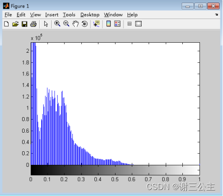
** Here's number one (2) Code of topic .** Yes gray Carry out piecewise linear transformation
Image1=im2double(imread('fj.jpg'));
gray=rgb2gray(Image1);
imhist(gray);
[h,w]=size(gray);
NewImage1=zeros(h,w);
a=80/256; b=180/256; c=30/256; d=220/256;
for x=1:w
    for y=1:h
        if gray(y,x)<a
            NewImage1(y,x)=gray(y,x)*c/a;
        elseif gray(y,x)<b
            NewImage1(y,x)=(gray(y,x)-a)*(d-c)/(b-a)+c;
        else
            NewImage1(y,x)=(gray(y,x)-b)*(255-d)/(255-b)+d;
        end
    end
end
figure,imshow(NewImage1),title(' Piecewise linear transformation ');
The obtained piecewise linear transformation is shown in the figure below :
** Here's number one (3) Code of topic .** Yes gray Histogram equalization ;
NewImage2=histeq(gray);
figure,imshow(NewImage2),title(' Histogram equalization ');
The histogram equalization diagram obtained is as follows :
** Here's number one (4) Code of topic .** Yes gray Pseudo color enhancement
NewImage3=zeros(h,w,3);
for x=1:w
    for y=1:h
        if gray(y,x)<64/256
            NewImage3(y,x,1)=0;
            NewImage3(y,x,2)=4*gray(y,x);
            NewImage3(y,x,3)=1;
        elseif gray(y,x)<128/256
            NewImage3(y,x,1)=0;
            NewImage3(y,x,2)=1;
            NewImage3(y,x,3)=2-4*gray(y,x);
        elseif gray(y,x)<192/256
            NewImage3(y,x,1)=4*gray(y,x)-2;
            NewImage3(y,x,2)=1;
            NewImage3(y,x,3)=0;
        else
            NewImage3(y,x,1)=1;
            NewImage3(y,x,2)=4-4*gray(y,x);
            NewImage3(y,x,3)=0;
        end
    end
end
figure,imshow(NewImage3);
The image of pseudo color enhancement is as follows :
** Here's number one (5) Code of topic .** Yes gray Add noise and smooth
noiseIsp=imnoise(gray,'salt & pepper',0.1);
noiseIg=imnoise(gray,'gaussian');
result1=medfilt2(noiseIsp);
result2=medfilt2(noiseIg);
figure;
subplot(121),imshow(result1),title(' Salt and pepper noise 3×3 median filtering ');
subplot(122),imshow(result2),title(' Gaussian noise 3×3 median filtering ');
The figure with noise added and smoothed is as follows :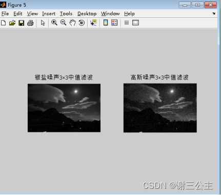
Here's number one (6) Code of topic . The ministry requires that gray utilize Sobel Operator sharpening
H1=[-1 -2 -1;0 0 0;1 2 1];
H2=[-1 0 1;-2 0 2;-1 0 1];
R1=imfilter(gray,H1);
R2=imfilter(gray,H2);
edgeImage=abs(R1)+abs(R2);
sharpImage=gray+edgeImage;
figure;
subplot(121),imshow(edgeImage),title('Sobel Gradient image ');
subplot(122),imshow(sharpImage),title('Sobel sharpen image ');
obtain Sobel The sharpened graph of the operator is as follows :
2. Expanded content in experimental requirements
(1) Transform the parameters for the above processing , Check the processing effect ;
(2) Change the pseudo color enhancement method to hot metal coding or rainbow coding ;
(3) Design different smoothing filters 、 Sharpening filtering method , Check the processing effect ;
(4) Self design method , Realize the color image enhancement processing .
The following is the expansion (1) Code of topic . Processing transformation parameters , Check the processing effect
( A little , Refer to the previous part of the code , Because of too much , Don't put it up again )
The figure of transformation parameters is as follows :


The following is the expansion (2) Code of topic . This topic requires changing the pseudo color enhancement method to hot metal coding or rainbow coding .
Rainbow code :
Image1=imread('lotus.bmp');

% Convert to grayscale
gray=rgb2gray(Image1);
[h,w]=size(gray);
% Matrix of the new image
NewImage3=zeros(h,w,3);
for x=1:h
    for y=1:w
        if gray(x,y)<96
        NewImage3(x,y,1)=0;
        elseif gray(x,y)<128
        NewImage3(x,y,1)=255*(gray(x,y)-96)/32;
        else
        NewImage3(x,y,1)=255;
        end
    end
end
for x=1:h
    for y=1:w
        if gray(x,y)<32
        NewImage3(x,y,2)=0;
        elseif gray(x,y)<64
        NewImage3(x,y,2)=255*(gray(x,y)-32)/32;
        elseif gray(x,y)<128
        NewImage3(x,y,2)=255;
        elseif gray(x,y)<192
        NewImage3(x,y,2)=255*(192-gray(x,y))/64;
        else
        NewImage3(x,y,2)=255*(gray(x,y)-192)/64;
        end
    end
end
for x=1:h
    for y=1:w
        if gray(x,y)<32
        NewImage3(x,y,3)=255*gray(x,y)/32;
        elseif gray(x,y)<64
        NewImage3(x,y,3)=255;
        elseif gray(x,y)<96
        NewImage3(x,y,3)=255*(96-gray(x,y))/32;
        elseif gray(x,y)<192
        NewImage3(x,y,3)=0;
        else
        NewImage3(x,y,3)=255*(gray(x,y)-192)/64;
        end
    end
end
imshow(NewImage3),title(' Rainbow code ')
The figure of color image transformation to rainbow coding is as follows :
The following is the expansion (3) Code of topic . This topic designs different smoothing filters 、 Sharpening filtering method , Check the processing effect .
1. be based on Robert Cross gradient image sharpening :
I = imread('fj.jpg');
imshow(I);
I = double(I); %  Convert to double type , This saves negative values , otherwise uint8 Type will cut off the negative value
w1 = [-1 0; 0 1]
w2 = [0 -1; 1 0]
G1 =  imfilter(I, w1, 'corr', 'replicate'); %  Fill the boundary repeatedly
G2 =  imfilter(I, w2, 'corr', 'replicate');
G = abs(G1) + abs(G2); %  Calculation Robert gradient
figure, imshow(G, []);
figure, imshow(abs(G1), []);
figure, imshow(abs(G2), []);
2.  Smoothing filter code
I = imread('fj.jpg');
J1=imnoise(I,'salt & pepper',0.02); % Plus mean value is 0, The variance of 0.02 Salt and pepper noise
J2=imnoise(I,'gaussian',0.02); % Plus mean value is 0, The variance of 0.02 Gaussian noise of .
g1=rgb2gray(J1);
g2=rgb2gray(J2);
figure('units','normalized','position',[0 0 1 1]);
subplot(2,4,1),imshow(J1),xlabel(' Salt and pepper noise '); % Displays a salt and pepper noise image
subplot(2,4,2),imshow(J2),xlabel(' Gaussian noise '); % Gaussian noise image is displayed

% %   Neighborhood averaging   neighborhood averaging

% imfilter  It can carry out multi-dimensional image (RGB etc. ) Spatial filtering , And there are many optional parameters
% filter2 / medfilt2  Only two-dimensional images ( grayscale ) Spatial filtering ,
%  The result types of the two functions are different , Only need I1=filter2(h,I) Followed by I1=uint8(I1) Do type conversion , The result is the same .

K1 = filter2(fspecial('average',3),g1); %  Salt and pepper noise  3*3  Template smoothing filtering
K2 = filter2(fspecial('average',11),g1);
k3 = imfilter(I,fspecial('average',3),'replicate');
K4 = filter2(fspecial('average',3),g2); %  Gaussian noise  3*3  Template smoothing filtering

subplot(2,4,3),imshow(uint8(K1)),xlabel({
    ' Salt and pepper noise ';'3*3  Template smoothing filtering '});
subplot(2,4,4),imshow(uint8(K1)),xlabel({
    ' Salt and pepper noise ';'11*11  Template smoothing filtering '});
subplot(2,4,5),imshow(k3),xlabel('3*3 imfilter Spatial filtering ');
subplot(2,4,6),imshow(uint8(K4)),xlabel(' Gaussian noise  3*3  Template smoothing filtering ');

%  median filtering
I1= medfilt2(g1,[3,3]); %  The image with salt and pepper noise is 5×5 Square window median filter
I2= medfilt2(g2,[3,3]); %  For images with Gaussian noise 5×5 Square window median filter

subplot(2,4,7),imshow(I1),xlabel({
    ' Salt and pepper noise ';'3*3  median filtering '});
subplot(2,4,8),imshow(I2),xlabel({
    ' Gaussian noise ';'3*3  median filtering '});
Get self-designed based on smooth filtering 、 The figure of sharpened filtered image is as follows :

( Sharpening filter )
( Smooth filtering )
** The following is the expansion (4) Code of topic .** Self design method , Realize the color image enhancement processing .
Yes RGB Image direct linear transformation for color enhancement
clear;clc;
rgb  = imread('fj.jpg');
[o p q]=size(rgb);
r(:,:,1)=rgb(:,:,1);
r(:,:,2)=zeros(o,p);
r(:,:,3)=zeros(o,p);
r=r*1.4;
g(:,:,2)=rgb(:,:,2);
g(:,:,1)=zeros(o,p);
g(:,:,3)=zeros(o,p);
g=g*1.4;
b(:,:,3)=rgb(:,:,3);
b(:,:,2)=zeros(o,p);
b(:,:,1)=zeros(o,p);
b=b*1.4;
rgb_new(:,:,1)=r(:,:,1);
rgb_new(:,:,2)=g(:,:,2);
rgb_new(:,:,3)=b(:,:,3);
figure;
subplot(121);imshow(rgb);title(' original rgb Images ');
%subplot(231);imshow(r);title(' Red component image ');
%subplot(232);imshow(g);title(' Green component image ');
%subplot(233);imshow(b);title(' Blue component image ');
subplot(122);imshow(rgb_new);title(' After enhancement rgb Images ');
The picture of color image enhancement is as follows :
Four 、 Summary of the experiment
Further master image processing tools Matlab, Be familiar with based on Matlab Image processing function . Through experiments, I have a deep understanding of various image enhancement methods , For example, master will Image1 Grayscale to gray, Statistics and display its gray histogram ; Yes gray Carry out piecewise linear transformation ; Yes gray Histogram equalization ; Yes gray Pseudo color enhancement ; Yes gray Add noise and smooth ; Yes gray utilize Sobel Operator sharpening method and so on , It lays a foundation for further study .
边栏推荐
- Buckle practice - 14 simplified path
- OLED循环显示图片文字
- Ethernet development and testing, have you done this step right (2)
- CentOS7.9安装MySQL8详细步骤
- 力扣练习——18 前 K 个高频元素
- Five reasons why developers use helix QAC to achieve static code test compliance
- 直流电机控制系统设计
- Buckle practice - 15 rain
- LCD1602显示按键位置
- Reinforcement learning (I)
猜你喜欢

Super easy to use screenshot software snipaste (including installation package), how to set snipaste to start automatically

力扣练习——20 接雨水 II

Original error was: DLL load failed while importing _ multiarray_ Umath: the specified module cannot be found

0715-铁矿石跌10%

力扣练习——14 简化路径
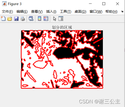
实验五 图像分割与描述

注册表实用技能【持续更新】

【vulnhub】FIVE86: 1

损失函数与极大似然估计的联系 | 交叉熵的理解

IP静态路由综合实验
随机推荐
There is only one day left to prepare for the examination of Guangxi Second Construction Engineering Co., Ltd. the first three pages of the examination of second-class cost engineer came and raised sc
skywalking测试环境部署实战
Question v: hannnnah_ j’s Biological Test
交通灯 单片机课程设计
Using off heap memory
JVM 问题定位工具
力扣练习——17 任务调度器
一文读懂软件测试的常见分类
力扣练习——和至少为 K 的最短子数组
Algorithm In Interview
基于ADC0832的电位器数值显示
Reinforcement learning (I)
实验二 图像增强
Five reasons why developers use helix QAC to achieve static code test compliance
架构师进阶,微服务设计与治理的 16 条常用原则
Ethernet development and testing, have you done this step right (3)
11 digits of mobile phone number and format verification rules
Usage and difference between sizeof and strlen in C language
Deployment practice of skywalking test environment
(手工)【sqli-labs42、43】POST注入、堆叠注入、错误回显、字符型注入