当前位置:网站首页>Deep learning parameter initialization (II) Kaiming initialization with code
Deep learning parameter initialization (II) Kaiming initialization with code
2022-07-19 12:21:00 【Xiaoshu Xiaoshu】
Catalog
3、 ... and 、Kaiming Initialization assumptions
Four 、Kaiming Simple formula derivation of initialization
5、 ... and 、Pytorch Realization
Deep learning parameter initialization series :
( One )Xavier initialization With code
( Two )Kaiming initialization With code
One 、 Introduce
Kaiming Initialize the paper address :https://arxiv.org/abs/1502.01852
Xavier Initialize at ReLU Layer performance is not good , The main reason is relu The layer maps negative numbers to 0, Affect the overall variance . and Xavier The activation function applicable to the initialization method is limited : Requirements about 0 symmetry ; linear . and ReLU The activation function does not meet these conditions , Experiments can also verify Xavier Initialization does not apply to ReLU Activation function . So he Kaiming has made improvements , Put forward Kaiming initialization , At first, it was mainly used in computer vision 、 Convolution network .
Two 、 Basic knowledge of
1. Suppose that random variables X And random variables Y Are independent of each other , Then there are
 (1)
(1)
2. A formula for finding variance by expectation , The expectation that the variance is equal to the square minus the square of the expectation .
 (2)
(2)
3. Independent variable product formula
 (3)
(3)
4. Continuous random variable X The probability density function of is f(x), If integral converges absolutely , The expected formula is as follows :
 (4)
(4)
3、 ... and 、Kaiming Initialization assumptions
And Xavier Initialization is similar ,Kaiming Initialization also applies Glorot Conditions , That is, our initialization strategy should make the activation value of each layer consistent with the variance of the state gradient in the propagation process ;Kaiming The initialized parameters still meet the mean value of 0, And the average weight during the update process has always been 0.
And Xavier Initialize different ,Kaiming Initialization no longer requires that the average output of each layer be 0( because Relu Such an activation function cannot be done ); Of course, it is no longer required f′(0)=1.
Kaiming In the initialization , Forward propagation and back propagation use their own initialization strategies , But ensure that the variance of each layer in forward propagation and the variance of gradient in back propagation are 1.
Four 、Kaiming The initialization of the Simple formula derivation
We use convolution to derive , And the activation function uses ReLU.
1. Forward propagation
For a layer of convolution , Yes :
 (5)
(5)
among  Is the output before activating the function ,
 Is the number of weights ,
 Weight. ,
 It's input .
according to (3) type , Can be (4) The formula is deduced as :
![Var(y_{i})=n_{i}[Var(w_{i})Var(x_{i})+Var(w_{i})(E(x_{i}))^{2}+(E(w_{i}))^{2}Var(x_{i})]](http://img.inotgo.com/imagesLocal/202207/19/202207171612297823_47.gif) (6)
(6)
Based on assumptions  , however It is the upper layer that passes ReLU Got , therefore
  , be :
![Var(y_{i})=n_{i}[Var(w_{i})Var(x_{i})+Var(w_{i})(E(x_{i}))^{2}]](http://img.inotgo.com/imagesLocal/202207/19/202207171612297823_22.gif)
 (7)
(7)
adopt (2) Type available  , be (7) The formula is deduced as :
 (8)
(8)
According to the expectation formula (4), Pass the first  Layer output to find this expectation , We have
  , among
  Express ReLU function .
 (9)
(9)
among  Represents the probability density function , because
  When
When  , So you can remove less than 0 The range of , And greater than 0 When
  , Can be launched :
 (10)
(10)
because  It is assumed that 0 It is symmetrically distributed around and the mean value is 0, therefore
  Also in 0 The nearby distribution is symmetrical , And the mean is 0( Assume here that the offset is 0), be
 (11)
(11)
therefore  The expectation is :

 (12)
(12)
According to the formula (2), because Our expectations are equal to 0, So there is :

The type (12) Derived as :
 (13)
(13)
take (13) Type in (8) type :
 (14)
(14)
Carry out forward propagation from the first floor , The variance of a certain layer can be obtained as :

there  Is the input sample , We will normalize it , therefore
  , Now let the output variance of each layer be equal to 1, namely :


So when it spreads forward ,Kaiming The implementation of initialization is the following uniform distribution :
![W\sim U[-\sqrt{\frac{6}{n_{i}}},\sqrt{\frac{6}{n_{i}}}]](http://img.inotgo.com/imagesLocal/202207/19/202207171612297823_40.gif)
Gaussian distribution :
![W\sim N[0,\frac{2}{n_{i}}]](http://img.inotgo.com/imagesLocal/202207/19/202207171612297823_7.gif)
2. Back propagation
Because back propagation
 (15)
(15)
among  Means that the loss function takes its derivative .
  Is the parameter
according to (3) type :

![=\hat{n}[Var(\hat{w})Var(\Delta y_{i})+Var(\hat{w_{i}})(E\Delta y_{i})^{2}+Var(\Delta y_{i})(E\hat{w}_{i})^{2}]](http://img.inotgo.com/imagesLocal/202207/19/202207171612297823_1.gif)

among  Indicates the number of output channels during back propagation , At last, it comes to


So back propagation ,Kaiming The implementation of initialization is the following uniform distribution :
![W\sim U[-\sqrt{\frac{6}{\hat{n}_{i}}},\sqrt{\frac{6}{\hat{n}_{i}}}]](http://img.inotgo.com/imagesLocal/202207/19/202207171612297823_37.gif)
Gaussian distribution :
![W\sim N[0,\frac{2}{\hat{n}_{i}}]](http://img.inotgo.com/imagesLocal/202207/19/202207171612297823_39.gif)
5、 ... and 、Pytorch Realization
import torch

class DemoNet(torch.nn.Module):
    def __init__(self):
        super(DemoNet, self).__init__()
        self.conv1 = torch.nn.Conv2d(1, 1, 3)
        print('random init:', self.conv1.weight)
        '''
            kaiming  The initialization method obeys uniform distribution  U~(-bound, bound), bound = sqrt(6/(1+a^2)*fan_in)
            a  Is the slope of the negative half axis of the activation function ,relu  yes  0
            mode-  Optional  fan_in  or  fan_out, fan_in  When propagating forward , The variance is consistent ; fan_out  When making back propagation , The variance is consistent
            nonlinearity-  Optional  relu  and  leaky_relu , The default value is  . leaky_relu
        '''
        torch.nn.init.kaiming_uniform_(self.conv1.weight, a=0, mode='fan_out')
        print('xavier_uniform_:', self.conv1.weight)

        '''
            kaiming  The initialization method obeys the normal distribution , This is a  0  The normal distribution of the mean ,N~ (0,std), among  std = sqrt(2/(1+a^2)*fan_in)
            a  Is the slope of the negative half axis of the activation function ,relu  yes  0
            mode-  Optional  fan_in  or  fan_out, fan_in  When propagating forward , The variance is consistent ;fan_out  When making back propagation , The variance is consistent
            nonlinearity-  Optional  relu  and  leaky_relu , The default value is  . leaky_relu
        '''
        torch.nn.init.kaiming_normal_(self.conv1.weight, a=0, mode='fan_out')
        print('kaiming_normal_:', self.conv1.weight)


if __name__ == '__main__':
demoNet = DemoNet()边栏推荐
- 【C# wpf】个人网盘练习项目总结
- HCIP(4)
- 延迟加载JS的方式
- Familiar with nestjs (beginner)
- C# . Net Yunnan rural credit national secret signature (SM2) brief analysis
- Baidu document translation API
- Mysql-1366 - Incorrect string value: ‘\xE5\xBC\xA0\xE4\xB8\x89‘ for column ‘userName‘ at row 1
- 阿趣的思考
- Leetcode 150. Evaluation of inverse Polish expression
- How to apply applet container technology to develop hybrid app
猜你喜欢

LeetCode_ 17_ Letter combination of telephone number

HCIP(4)
C语言绘画示例-进度条

Travail du quatrième jour

Use native JS to realize the function of selecting all buttons, which is simple and clear
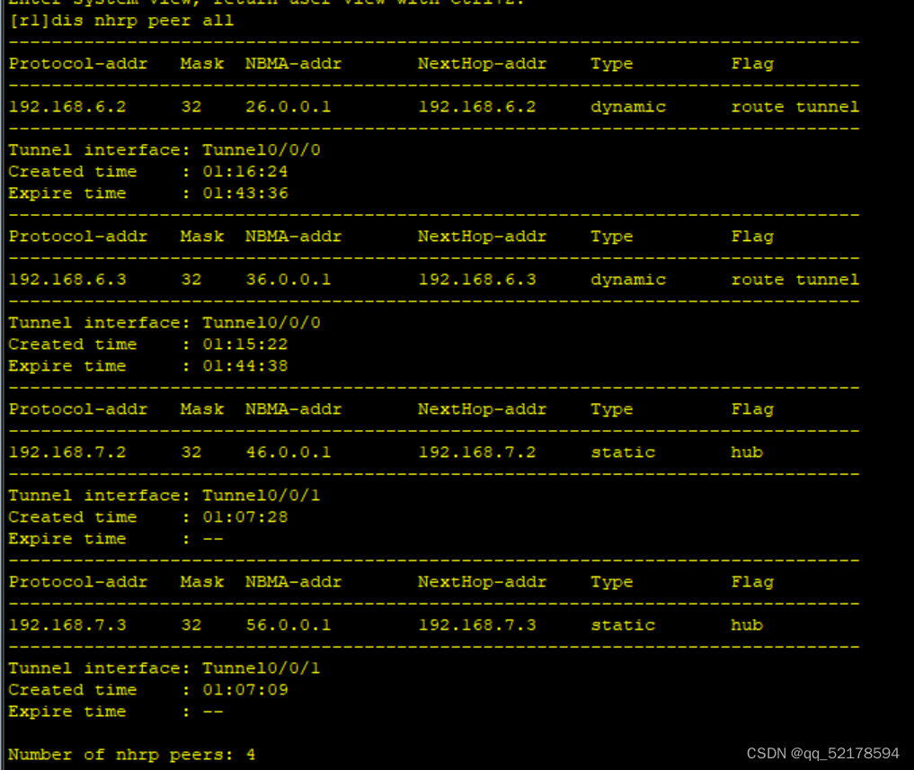
MGRE 环境下配置OSPF实验
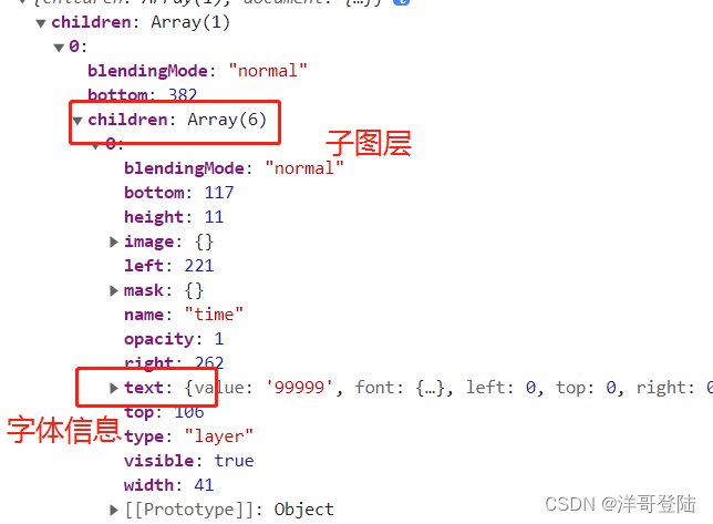
psd.js 解析PSD文件

getchar()
![[MySQL] add, delete, check and modify MySQL (Advanced)](/img/56/684204c509d3ce8db1397709216db7.png)
[MySQL] add, delete, check and modify MySQL (Advanced)
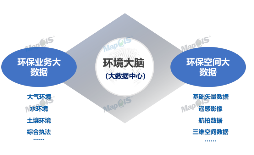
Focus on the new track of green development - release of MAPGIS intelligent environmental protection solution
随机推荐
LeetCode_ 17_ Letter combination of telephone number
PPPoE拨号上网
Wi Fi sensing technology and practice based on channel state information
zabbix-snmp监控
[shutter] dart: some features that cannot be ignored
STL string input / output overload
Linux下MySQL的安装与使用
Talk about the redis cache penetration scenario and the corresponding solutions
Genesis and bluerun ventures have in-depth exchanges
3. Golang string type
es安装ik分词器
第四天作业
2022安全员-C证上岗证题目及答案
Research on downlink spectrum efficiency of 6G space earth integrated network high altitude platform base station
李宏毅《机器学习》|1. Introduction of this course(机器学习介绍)
HCIP(4)
SwiftUI 颜色教程大全之中创建自定义调色板
STL string input / output overload 1
Use native JS to realize the function of selecting all buttons, which is simple and clear
C语言绘画示例-进度条