当前位置:网站首页>Convolution structure and its calculation
Convolution structure and its calculation
2022-07-18 20:00:00 【Grass in the crack of the wall】
List of articles
Convolution structure and its calculation
Convolution and its parameter design

Local connection : Vision is local , Give full consideration to domain information , Locally dense links
Weight sharing : Meizu weight extraction image is a feature of China
The response degree reduces the number of parameters 、 Avoid overfitting 
1D The above figure is used in natural language processing 
2D Typical use in image 

3D Convolution will 3 Dimensional filters are applied to datasets , And the filter will 3 Direction (x, y, z) Move to compute low-level features . Their output shape is 3 Dimensional volume space , For example, cube or box . They help video ,3D Event detection in medical images . They are not limited to 3d Space , It can also be applied to 2d Spatial input ( Such as images ).


Conv2D Class dilation_ rate Parameter is 2- Tuples , Used to control the expansion rate of expansion convolution .
Convolution optimization


Convolution back propagation 3
Convolution back propagation 4
Convolution back propagation 5
Winograd
Computational complexity 
computing method 
shortcoming :
●Depthwise conv Its advantage is not obvious .
● stay tile When you're older ,Winograd The method does not apply ,inverse transform Computational overhead offsets Winograd Computing savings .
●Winograd There will be errors .
Pooling
● Pooling is to use the overall statistical characteristics of adjacent outputs at a certain location to replace the output of the network at that location .
● Pooling (POOL) yes A down sampling operation , It is usually applied after convolution , The convolution layer performs some spatial invariance . among , The largest pool and the average pool are special types of pools , Take the maximum and average values respectively . Copyright poor heart College
Max Pooling
Average Pooling
Common methods of convolution calculation
● The sliding window : The calculation is slow , In general, do not use .
●im2col: Mainstream computing frameworks include Caffe, MXNet And so on . This method transforms the whole convolution process into GEMM The process ,GEMM In all kinds of BLAS The library is extremely optimized , Generally speaking , Faster .
●FFT: Fourier transform and fast Fourier transform are calculation methods often used in classical image processing , however , stay ConvNet Usually , Mainly because of ConvNet Convolution templates in are usually small , for example 3x3 etc. , In this case ,FFT The time cost is even greater .
●Winograd: Winograd Methods are shown and have great advantages , at present CUDNN This method is used to calculate convolution in .
Classical convolutional neural network model structure
LeNet-5

LeNet-5 It contains seven layers , Input... Is not included , Each layer contains trainable parameters ( The weight ), The input data used at that time was 32*32 Pixel image . The following is a layer by layer introduction LeNet- 5 Structure , also , The convolution layer will be Cx Express , The sub sampling layer is labeled Sx, The fully connected layer is marked Fx, among x It's a layer index .
AlexNet

AlexNet Yes 6 Billion parameters and 650000 Neurons , contain 5 Convolution layers ,3 All connection layers
VGG

By a very long 3 \times33x3 Convolution sequence , Interspersed 2 \times 22x2 Pooled layer , And finally 3 All connection layers .
GoogleNet
Inception That is, multiple convolution or pooling operations , Put them together and assemble them into a network module , When designing neural network, the whole network structure is assembled in modules . The module is shown in the figure below 
In networks that do not use this method , We often only use one operation at a layer , Such as convolution or pooling , And the convolution kernel size of convolution operation is also fixed . however , In practice , In pictures of different scales , Convolution kernels of different sizes are required , This can make the performance best , Or or , For the same picture , The performance of convolution kernels of different sizes is different , Because their feelings are different . therefore , We hope to let the network choose by itself ,Inception Can meet such needs , One Inception The module provides a variety of convolution kernel operations in parallel , In the process of training, the network selects and uses itself by adjusting parameters , meanwhile , Because pooling operations are required in the network , Therefore, the pooling layer is also added to the network in parallel .
GoogLeNet The overall network structure is shown in the figure below 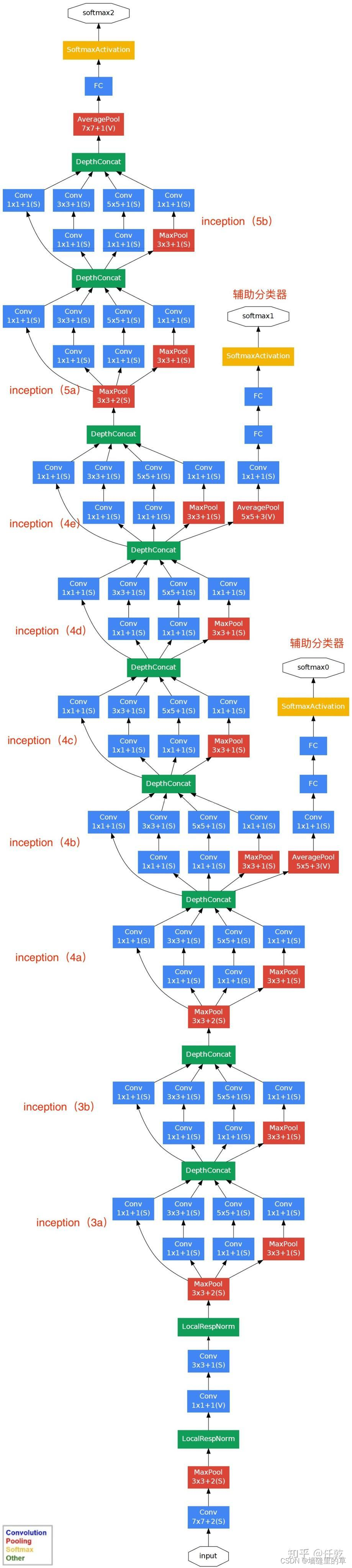
ResNet


Because the residual is usually small , Learning is less difficult . However, we can analyze this problem from the perspective of Mathematics , First, the residual element can be expressed as :
among Xl and Xl+1 They represent the... Respectively l Input and output of residual units , Note that each residual element generally contains a multi-layer structure .F Is the residual function , Represents the learned residuals , and h(xl)=xl Represents identity mapping ,f yes ReLU Activation function . Based on the above formula , We find that from the shallow l To the deep L The characteristics of learning are :
Using chain rules , The gradient of the reverse process can be obtained :
The first factor of the formula  The expressed loss function reaches L Gradient of , In parentheses 1 It shows that the short circuit mechanism can propagate the gradient losslessly , The other residual gradient needs to go through a process with weights The layer , The gradient is not passed directly . The residual gradient is not so coincidental. It's all -1, And even if it's small , Yes 1 The existence of does not cause the gradient to disappear . So residual learning will be easier .
The network structure is as follows 
边栏推荐
猜你喜欢

leetcode 45. Jump Game II (dp)

Vivado Ethernet interface (sgmii to gmii interface)

The admission list of the junior class of the University of science and technology of China was announced: Zhejiang is crazy about winning 30% of the places, and there are 4 people in Xuejun middle sc
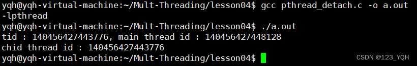
5.线程分离

Small program development of private forum circle community

老外还停留在20年前

电力系统经济调度(Matlab完整代码实现)

Leetcode's 82nd biweekly match
HCIA summary

Deadlock prevention, deadlock avoidance, deadlock detection
随机推荐
leetcode 45. Jump Game II (dp)
FIFO signal simulation of internal IP core based on FPGA
6.线程取消
Part II FPGA digital signal processing_ Verilog design of parallel FIR filter
Horizon 8 测试环境部署(8): App Volumes Managers 负载均衡配置
The 20th anniversary of Beijing Hyundai: Streamline product layout and strive to achieve 520000 vehicles by 2025
12. Quick sort
leetcode 43. String multiplication (string + simulation)
PSIM simulation model construction of buck circuit (II) (use of transfer function module)
全员满分!中国队IMO达成四连冠,大比分领先第二名韩国
Musk's 76 year old father and stepdaughter have children. Huaqiangbei has another chip IPO. The former vice president of ant has joined AI pharmaceutical. Today, more big news is here
安卓 Day 26 :数据库Two
Ci521 domestic 13.56MHz reader chip replaces cv520 compatible
4.连接已终止的线程(回收线程)
[LeetCode]剑指 Offer 39. 数组中出现次数超过一半的数字
处理数字用中文表示
Basic use of JUC
Nc20583 [sdoi2016] gear
Chapter I FPGA digital signal processing_ Digital mixing (NCO and DDS)
分享不停,踏浪前行 | 开发者说·DTalk 年中鉴赏