当前位置:网站首页>Mxnet network model of show me the code (III)
Mxnet network model of show me the code (III)
2022-07-19 01:52:00 【tissar】
Show Me the Code And MXNet A network model ( 3、 ... and )
LeNet yes 1986 Model published in .
A network model

| The network layer | Network type | Output data type | Training parameters | The front floor |
|---|---|---|---|---|
| Input | 1x28x28 | |||
| 1-Conv2D | Convolution layer | 6x28x28 | 6x(1x5x5+1)=156 | Input |
| 1-Activation | Activation layer | 6x28x28 | 1-Conv2D | |
| 1-MaxPool2D | Pooling layer | 6x14x14 | 1-Activation | |
| 2-Conv2D | Convolution layer | 16x10x10 | 16x(6x5x5+1)=2416 | 1-MaxPool2D |
| 2-Activation | Activation layer | 16x10x10 | 2-Conv2D | |
| 2-MaxPool2D | Pooling layer | 16x5x5 | 2-Activation | |
| 3-Dense | Full connection | 120 | 120x(16x5x5+1)=48120 | 2-MaxPool2D |
| 3-Activation | Activation layer | 120 | 3-Dense | |
| 4-Dense | Full connection | 84 | 84x(120+1)=10164 | 3-Activation |
| 4-Activation | Activation layer | 84 | 4-Dense | |
| 5-Dense | Full connection | 10 | 10x(84+1)=850 | 4-Activation |
| Statistics | 61706 |
Because the full connection layer takes up most of the training parameters (95.83%), The convolution layer consumes more computing power than the full connection layer . therefore , Some people say “ The whole connection layer is responsible for the parameter part , The convolution layer is responsible for the calculation part ”.
Show me the code!
Explain , The implementation here is the same as the original LeNet Not the same. . The original activation function is Sigmoid, And pooling is average pooling .
MXNet 1.5.1
# -*- coding: utf-8 -*-

import logging
import struct
import gzip
import numpy as np
import mxnet as mx

logging.getLogger().setLevel(logging.DEBUG)

#  Batch size
batch_size = 32
#  The number of study rounds
train_epoch = 20
#  Sample path
resource_path = "fashion-mnist/"

''' ************************************************************ *  Data preparation  ************************************************************ '''
#  Define functions to read data
def read_data( label_url, image_url ):
    with gzip.open( label_url ) as flbl:
        #  Read in label file header
        magic, num = struct.unpack(">II", flbl.read(8))
        #  Read the label content
        label = np.frombuffer( flbl.read(), dtype = np.uint8 )
    with gzip.open( image_url, 'rb' ) as fimg:
        #  Read in the image file header ,rows and cols All are 28
        magic, num, rows, cols = struct.unpack( ">IIII", fimg.read(16) )
        #  Read image content
        image = np.frombuffer( fimg.read(), dtype = np.uint8 )
        #  Set to the correct array format
        image = image.reshape( len(label), 1, rows, cols )
        #  Normalize to  0~1
        image = image.astype( np.float32 ) / 255.0
    return (label, image)

#  Read in the data
#  Pay attention to the path
( train_lbl, train_img ) = read_data(
        resource_path + 'train-labels-idx1-ubyte.gz',
        resource_path + 'train-images-idx3-ubyte.gz'
        )
( eval_lbl , eval_img  ) = read_data(
        resource_path + 't10k-labels-idx1-ubyte.gz',
        resource_path + 't10k-images-idx3-ubyte.gz'
        )

#  iterator
train_iter = mx.io.NDArrayIter( train_img, train_lbl, batch_size, shuffle=True )
eval_iter  = mx.io.NDArrayIter( eval_img , eval_lbl , batch_size )  #  The validation set can be omitted shuffle

''' ************************************************************ *  Define the neural network model  ************************************************************ '''
#  Input layer
net = mx.sym.var( 'data' )
#  The first 1 Layer hidden layer
net = mx.sym.Convolution   (data=net, name='layer1_conv', num_filter=6, kernel=(5,5), pad=(2,2))
net = mx.sym.Activation    (data=net, name='layer1_act' , act_type='relu')
net = mx.sym.Pooling       (data=net, name='layer1_pool', kernel=(2,2), stride=(2,2), pool_type='max')
#  The first 2 Layer hidden layer
net = mx.sym.Convolution   (data=net, name='layer2_conv', num_filter=16, kernel=(5,5))
net = mx.sym.Activation    (data=net, name='layer2_act' , act_type='relu')
net = mx.sym.Pooling       (data=net, name='layer2_pool', kernel=(2,2), stride=(2,2), pool_type='max')
#  The first 3 Layer hidden layer
net = mx.sym.Flatten       (data=net, name='flatten')       #  Flatten the image
net = mx.sym.FullyConnected(data=net, name='layer3_fc'  , num_hidden=120)
net = mx.sym.Activation    (data=net, name='layer3_act' , act_type='relu')
#  The first 4 Layer hidden layer
net = mx.sym.FullyConnected(data=net, name='layer4_fc'  , num_hidden=84)
net = mx.sym.Activation    (data=net, name='layer4_act' , act_type='relu')
#  Output layer
net = mx.sym.FullyConnected(data=net, name='layer5_fc'  , num_hidden=10)
net = mx.sym.SoftmaxOutput (data=net, name='softmax')       # Softmax It is also the activation layer

#  A network model
ctx = mx.gpu() if mx.test_utils.list_gpus() else mx.cpu()   #  Yes GPU Just use GPU
module = mx.mod.Module(symbol=net, context=ctx)

#  Network model visualization
# shape = {'data':(batch_size, 1, 28, 28)}
# mx.viz.print_summary(symbol=net, shape=shape)
# mx.viz.plot_network(symbol=net, shape=shape).view()

''' ************************************************************ *  Training neural network  ************************************************************ '''
#  Define evaluation criteria (Evaluation Metric)
eval_metrics = mx.metric.CompositeEvalMetric()
eval_metrics.add( mx.metric.Accuracy() );       #  Accuracy rate
eval_metrics.add( mx.metric.CrossEntropy() );   #  Cross entropy

print("start train...")

module.fit(
        train_data  = train_iter,               #  Training set
        eval_data   = eval_iter,                #  Verification set
        eval_metric = eval_metrics,             #  Evaluation criteria
        num_epoch   = train_epoch,              #  Number of training rounds
        initializer = mx.initializer.Xavier(),  # Xavier Initialization strategy
        optimizer   = 'sgd',                    #  Stochastic gradient descent algorithm
        optimizer_params = {

            'learning_rate': 0.01,              #  Learning rate
            'momentum': 0.9                     #  Inertia Momentum
            }
    )
INFO:root:Epoch[0] Train-accuracy=0.791900
INFO:root:Epoch[0] Train-cross-entropy=0.560617
INFO:root:Epoch[0] Time cost=5.205
INFO:root:Epoch[0] Validation-accuracy=0.860024
INFO:root:Epoch[0] Validation-cross-entropy=0.387932
INFO:root:Epoch[1] Train-accuracy=0.871650
INFO:root:Epoch[1] Train-cross-entropy=0.351662
INFO:root:Epoch[1] Time cost=5.167
INFO:root:Epoch[1] Validation-accuracy=0.883786
INFO:root:Epoch[1] Validation-cross-entropy=0.316452
…
INFO:root:Epoch[19] Train-accuracy=0.942633
INFO:root:Epoch[19] Train-cross-entropy=0.151282
INFO:root:Epoch[19] Time cost=5.186
INFO:root:Epoch[19] Validation-accuracy=0.907548
INFO:root:Epoch[19] Validation-cross-entropy=0.307947
MXNet 1.9.1
The above code , here we are MXNet 1.6.0 The version won't work .
Here are the new implementations .
import time
import struct
import gzip
import numpy as np
import matplotlib.pyplot as plt
import mxnet as mx
Set the batch size and CPU
batch_size = 32
device = mx.cpu(0)
Define function , Read the picture
def read_data( label_url, image_url ):
    with gzip.open( label_url ) as flbl:
        #  Read in label file header
        magic, num = struct.unpack( ">II", flbl.read(8) )
        label = np.frombuffer( flbl.read(), dtype = np.uint8 )
    with gzip.open( image_url, 'rb' ) as fimg:
        #  Read in the image file header ,rows and cols All are 28
        magic, num, rows, cols = struct.unpack( ">IIII", fimg.read(16) )
        #  Read image content
        image = np.frombuffer( fimg.read(), dtype = np.uint8 )
        #  Set to the correct array format
        image = image.reshape( num, 1, rows, cols )
        #  Normalize to  [-1,1]
        image = image.astype( np.float32 ) / 255.0
    return (label, image)
Reading data , Print dimension
( train_lbl, train_img ) = read_data(
    'fashion-mnist/train-labels-idx1-ubyte.gz',
    'fashion-mnist/train-images-idx3-ubyte.gz'
)
( eval_lbl , eval_img  ) = read_data(
    'fashion-mnist/t10k-labels-idx1-ubyte.gz',
    'fashion-mnist/t10k-images-idx3-ubyte.gz'
)
print("train:", type(train_img), train_img.shape, train_img.dtype)
print("eval: ", type(eval_img),  eval_img.shape,  eval_img.dtype )
train: <class ‘numpy.ndarray’> (60000, 1, 28, 28) float32
eval: <class ‘numpy.ndarray’> (10000, 1, 28, 28) float32
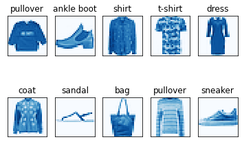
View data pictures
texts = (
    't-shirt', 'trouser', 'pullover', 'dress', 'coat',
    'sandal',  'shirt',   'sneaker',  'bag',   'ankle boot'
)
idxs = (0, 1, 2, 3, 4, 5, 7, 9, 14, 21)

for i in range(10):
    plt.subplot(2, 5, i + 1)
    idx = idxs[i]
    plt.xticks([])
    plt.yticks([])
    plt.title(texts[train_lbl[idx]])
    img = train_img[idx][0].astype( np.float32 )
    plt.imshow(img, interpolation='none', cmap='Blues')

plt.show()
Create a training iterator . This step sets the batch size and the random sorting of the training set .
train_data = mx.gluon.data.DataLoader(
    mx.gluon.data.ArrayDataset(train_img, train_lbl),
    batch_size=batch_size,
    shuffle=True
)
eval_data = mx.gluon.data.DataLoader(
    mx.gluon.data.ArrayDataset(eval_img, eval_lbl),
    batch_size=batch_size,
    shuffle=False
)
Define an evaluation class . use MXNet It's OK to bring your own , But I want to package show()
class UserMetrics(mx.metric.CompositeEvalMetric):
    def __init__(self, name='user', output_names=None, label_names=None):
        #  initialization PyTorch Parent class
        super().__init__(name=name, output_names=output_names, label_names=label_names)
        super().add( mx.metric.Accuracy() )
        super().add( mx.metric.CrossEntropy() )
    def reset(self):
        super().reset()
        self.tic = time.time()
    def show(self, epoch=0, tag='[ ]'):
        cost = time.time() - self.tic
        name, val = super().get()
        print("Epoch %2d: %s cost:%.1fs %s:%.3f, %s:%.3f"
              % ( epoch, tag, cost, name[0], val[0], name[1], val[1] )
        )
Defining network
#  Network type
net = mx.gluon.nn.HybridSequential()

#  Middle layer
net.add(
    #  first floor
    mx.gluon.nn.Conv2D( channels=6,  kernel_size=(5,5), strides=(1,1), padding=(2,2) ),
    mx.gluon.nn.Activation( 'relu' ),
    mx.gluon.nn.MaxPool2D( pool_size=(2,2) ),
    #  The second floor
    mx.gluon.nn.Conv2D( channels=16, kernel_size=(5,5), strides=(1,1), padding=(0,0) ),
    mx.gluon.nn.Activation( 'relu' ),
    mx.gluon.nn.MaxPool2D( pool_size=(2,2) ),
    #  The third level
    mx.gluon.nn.Dense( 120 ),
    mx.gluon.nn.Activation( 'relu' ),
    #  The fourth level
    mx.gluon.nn.Dense( 84 ),
    mx.gluon.nn.Activation( 'relu' )
)

#  Output layer
net.output = mx.gluon.nn.Dense( 10 )

#  initialization
net.initialize( init=mx.init.Xavier(), ctx=device )

#  Show the Internet
net.summary(mx.ndarray.zeros(shape=(1, 1, 28, 28), dtype=np.float32, ctx=device))

#  Symbolic acceleration
net.hybridize()

Loss function , Trainer , Evaluator
#  Loss function
loss_function = mx.gluon.loss.SoftmaxCrossEntropyLoss()
#  solver
optimizer = mx.optimizer.SGD( learning_rate=0.01, momentum=0.0, multi_precision=False )
#  Trainer
trainer = mx.gluon.Trainer( params=net.collect_params(), optimizer=optimizer )
#  Evaluator
metrics = UserMetrics()
Start training 20 epoch
for epoch in range(20):
    # train
    metrics.reset()
    for datas, labels in train_data:

        actual_batch_size = datas.shape[0]

        # split batch and load into corresponding devices
        datas  = mx.gluon.utils.split_and_load( datas,  [device] )
        labels = mx.gluon.utils.split_and_load( labels, [device] )

        # The forward pass and the loss computation
        with mx.autograd.record():
            outputs = [ net(data) for data in datas ]
            losses = [ loss_function(output, label) for output, label in zip(outputs, labels) ]

        # compute gradients
        for loss in losses:
            loss.backward()

        # update parameters
        trainer.step( batch_size=actual_batch_size )

        # update metric
        for output, label in zip(outputs, labels):
            metrics.update( preds=mx.ndarray.softmax(output, axis=1), labels=label )

    metrics.show( epoch=epoch, tag='[ train ]' )

    # eval
    metrics.reset()
    for datas, labels in eval_data:
        # split batch and load into corresponding devices
        datas  = mx.gluon.utils.split_and_load(datas,  [device])
        labels = mx.gluon.utils.split_and_load(labels, [device])
        # The forward pass
        outputs = [ net(data) for data in datas ]
        # update metric
        for output, label in zip(outputs, labels):
            metrics.update( preds=mx.ndarray.softmax(output, axis=1), labels=label )
    metrics.show( epoch=epoch, tag='[ eval ]' )
Epoch 0: [ train ] cost:8.0s accuracy:0.693, cross-entropy:0.847
Epoch 0: [ eval ] cost:0.6s accuracy:0.784, cross-entropy:0.588
Epoch 1: [ train ] cost:7.9s accuracy:0.805, cross-entropy:0.531
Epoch 1: [ eval ] cost:0.6s accuracy:0.837, cross-entropy:0.453
Epoch 2: [ train ] cost:7.9s accuracy:0.835, cross-entropy:0.452
Epoch 2: [ eval ] cost:0.6s accuracy:0.851, cross-entropy:0.420
…
Epoch 18: [ train ] cost:8.0s accuracy:0.908, cross-entropy:0.250
Epoch 18: [ eval ] cost:0.6s accuracy:0.896, cross-entropy:0.290
Epoch 19: [ train ] cost:8.0s accuracy:0.910, cross-entropy:0.244
Epoch 19: [ eval ] cost:0.6s accuracy:0.899, cross-entropy:0.273
边栏推荐
- 基于机器学习技术的无线小区负载均衡自优化
- fetch请求-简单记录
- errno详解
- Why do you spend 1.16 million to buy an NFT avatar in the library of NFT digital collections? The answer may be found by reviewing the "rise history" of NFT avatars
- 感通融合系统中保障公平度的时间与功率分配方法
- Why is opensea the absolute monopolist of NFT trading market?
- wkwebview白屏
- 字节二面:什么是伪共享?如何避免?
- Cannot find module ‘process‘ or its corresponding type declarations.
- 5G专网在智慧医疗中的应用
猜你喜欢

1章 性能平台GodEye源码分析-整体架构

面试官问:Redis 突然变慢了如何排查?

uniapp打包H5 空白页面 报错 Uncaught SyntaxError: Unexpected token ‘<‘

Solve the problem that Scala cannot initialize the class of native

开源项目丨 Taier 1.1 版本正式发布,新增功能一览为快

Frustratingly Simple Few-Shot Object Detection

袋鼠云数栈基于CBO在Spark SQL优化上的探索

温州大学X袋鼠云:高等人才教育建设,如何做到“心中有数”

Express project creation and its routing introduction

Redis+Caffeine两级缓存,让访问速度纵享丝滑
随机推荐
AVPlayer添加播放进度监听
0章 性能平台GodEye源码分析-课程介绍
温州大学X袋鼠云:高等人才教育建设,如何做到“心中有数”
蛟分承影,雁落忘归——袋鼠云一站式全自动化运维管家ChengYing(承影)正式开源
Owl Eyes: Spotting UI Display Issues via Visual Understanding
Cannot find module ‘process‘ or its corresponding type declarations.
Xcode11新建项目后的一些问题
【文献阅读】VAQF: Fully Automatic Software-Hardware Co-Design Framework for Low-Bit Vision Transformer
ViLT Vision-and-Language Transformer Without Convolution or Region Supervision
通感一体化融合的研究及其挑战
Neutralizing Self-Selection Bias in Sampling for Sortition
开源项目丨 Taier 1.1 版本正式发布,新增功能一览为快
Ansible
安全多方计算体系架构及应用思考
touchID 和 FaceID~1
面试官问:Redis 突然变慢了如何排查?
iPhone 各大机型设备号
Cento7 installs mysql5.5 and upgrades 5.7
爭奪存量用戶關鍵戰,助力企業構建完美標簽體系丨01期直播回顧
MapReduce环境准备