监督学习week 3: Logistic Regression optional_lab收获记录

目录

1.技巧one：利用布尔索引分别去画图    

2.注意：有关numpy

3.课程中define的loss和cost区别：

4.Cost Function for Logistic Regression     

5.compute_gradient_logistic   

6.Gradient Descent  

 7.Logistic Regression using Scikit-Learn

 ① Dataset

②Fit the model

③Make Predictions

④Calculate accuracy

8.To avoid the overfitting->Regularized Cost and Gradient Goals

        ①theory and formula​编辑

         ②Cost functions with regularization

        ③Gradient descent with regularization​编辑

1.技巧one：利用布尔索引分别去画图    

x_train = np.array([0., 1, 2, 3, 4, 5])
y_train = np.array([0,  0, 0, 1, 1, 1])
X_train2 = np.array([[0.5, 1.5], [1,1], [1.5, 0.5], [3, 0.5], [2, 2], [1, 2.5]])
y_train2 = np.array([0, 0, 0, 1, 1, 1])

pos = y_train == 1 #positive->注意：本处采用的是bool索引
neg = y_train == 0 #negeative

fig,ax = plt.subplots(1,2,figsize=(8,3))
#plot 1, single variable
ax[0].scatter(x_train[pos], y_train[pos], marker='x', s=80, c = 'red', label="y=1")
ax[0].scatter(x_train[neg], y_train[neg], marker='o', s=100,
     label="y=0", facecolors='none', edgecolors=dlc["dlblue"],lw=3)

ax[0].set_ylim(-0.08,1.1)
ax[0].set_ylabel('y', fontsize=12)
ax[0].set_xlabel('x', fontsize=12)
ax[0].set_title('one variable plot')
ax[0].legend()

#plot 2, two variables
plot_data(X_train2, y_train2, ax[1])
ax[1].axis([0, 4, 0, 4])
ax[1].set_ylabel('$x_1$', fontsize=12)
ax[1].set_xlabel('$x_0$', fontsize=12)
ax[1].set_title('two variable plot')
ax[1].legend()
plt.tight_layout()
plt.show()

2.注意：有关numpy

①一维数组的C_按列连接

②1/1+z(当z为矩阵的时候,运算的情况,依次对于每一个数都会进行操作) 

③NumPy has a function called exp(), which offers a convenient way to calculate the exponential ( 𝑒𝑧ez) of all elements in the input array (z).

3.课程中define的loss和cost区别：

Definition Note: In this course, these definitions are used:
Loss is a measure of the difference of a single example to its target value while the
Cost is a measure of the losses over the training set

4.Cost Function for Logistic Regression     

Note that the variables X and y are not scalar values but matrices of shape (𝑚,𝑛m,n) and (𝑚𝑚,) respectively, where 𝑛𝑛 is the number of features and 𝑚𝑚 is the number of training examples.

def compute_cost_logistic(X, y, w, b):
    """
    Args:
      X (ndarray (m,n)): Data, m examples with n features
      y (ndarray (m,)) : target values
      w (ndarray (n,)) : model parameters  
      b (scalar)       : model parameter"""
    m = X.shape[0]
    cost = 0.0
    for i in range(m):
        z_i = np.dot(X[i],w) + b
        f_wb_i = sigmoid(z_i)
        cost +=  -y[i]*np.log(f_wb_i) - (1-y[i])*np.log(1-f_wb_i)
             
    cost = cost / m
    return cost

5.compute_gradient_logistic   

def compute_gradient_logistic(X, y, w, b): 
    """
    Args:
      X (ndarray (m,n): Data, m examples with n features
      y (ndarray (m,)): target values
      w (ndarray (n,)): model parameters  
      b (scalar)      : model parameter
    Returns
      dj_dw (ndarray (n,)): The gradient of the cost w.r.t. the parameters w. 
      dj_db (scalar)      : The gradient of the cost w.r.t. the parameter b. 
    """
    m,n = X.shape
    dj_dw = np.zeros((n,))                           #(n,)
    dj_db = 0.

    for i in range(m):
        f_wb_i = sigmoid(np.dot(X[i],w) + b)          #(n,)(n,)=scalar
        err_i  = f_wb_i  - y[i]                       #scalar
        for j in range(n):
            dj_dw[j] = dj_dw[j] + err_i * X[i,j]      #scalar
        dj_db = dj_db + err_i
    dj_dw = dj_dw/m                                   #(n,)
    dj_db = dj_db/m                                   #scalar
        
    return dj_db, dj_dw  

6.Gradient Descent  

def gradient_descent(X, y, w_in, b_in, alpha, num_iters): 
    """
    Args:
      X (ndarray (m,n)   : Data, m examples with n features
      y (ndarray (m,))   : target values
      w_in (ndarray (n,)): Initial values of model parameters  
      b_in (scalar)      : Initial values of model parameter
      alpha (float)      : Learning rate
      num_iters (scalar) : number of iterations to run gradient descent
    Returns:
      w (ndarray (n,))   : Updated values of parameters
      b (scalar)         : Updated value of parameter 
    """
    J_history = []  # for graphing later
    w = copy.deepcopy(w_in)  #avoid modifying global w within function
    b = b_in
    
    for i in range(num_iters):
        dj_db, dj_dw = compute_gradient_logistic(X, y, w, b) # Calculate the gradient and update the parameters
        w = w - alpha * dj_dw   # Update Parameters using w, b, alpha and gradient             
        b = b - alpha * dj_db               
      
        if i<100000:      # prevent resource exhaustion 
            J_history.append( compute_cost_logistic(X, y, w, b) )   # Save cost J at each iteration

        if i% math.ceil(num_iters / 10) == 0:
            print(f"Iteration {i:4d}: Cost {J_history[-1]}   ")        # Print cost every at intervals 10 times or as many iterations if < 10
        
    return w, b, J_history         #return final w,b and J history for graphing

 7.Logistic Regression using Scikit-Learn

 ① Dataset

import numpy as np
X = np.array([[0.5, 1.5], [1,1], [1.5, 0.5], [3, 0.5], [2, 2], [1, 2.5]])
y = np.array([0, 0, 0, 1, 1, 1])

②Fit the model

        The code below imports the logistic regression model from scikit-learn. You can fit this model on the training data by calling fit function.

from sklearn.linear_model import LogisticRegression
lr_model = LogisticRegression()
lr_model.fit(X, y)

③Make Predictions

        see the predictions made by this model by calling the predict function.

y_pred = lr_model.predict(X)
print("Prediction on training set:", y_pred)

Prediction on training set: [0 0 0 1 1 1]

④Calculate accuracy

        calculate this accuracy of this model by calling the score function.

print("Accuracy on training set:", lr_model.score(X, y))

Accuracy on training set: 1.0

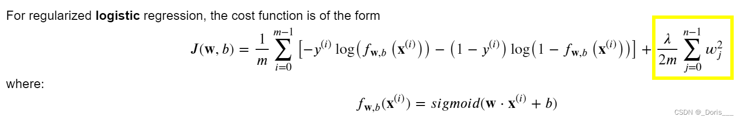
8.To avoid the overfitting->Regularized Cost and Gradient Goals

        ①theory and formula

         ②Cost functions with regularization

                （i）Cost function for regularized linear regression

                 不惩罚b

def compute_cost_linear_reg(X, y, w, b, lambda_ = 1):
    """
    Args:
      X (ndarray (m,n): Data, m examples with n features
      y (ndarray (m,)): target values
      w (ndarray (n,)): model parameters  
      b (scalar)      : model parameter
      lambda_ (scalar): Controls amount of regularization
    Returns:    total_cost (scalar):  cost 
    """
    m  = X.shape[0]
    n  = len(w)
    cost = 0.
    for i in range(m):
        f_wb_i = np.dot(X[i], w) + b                                   #(n,)(n,)=scalar, see np.dot
        cost = cost + (f_wb_i - y[i])**2                               #scalar             
    cost = cost / (2 * m)                                              #scalar  
 
    reg_cost = 0
    for j in range(n):
        reg_cost += (w[j]**2)                                          #scalar
    reg_cost = (lambda_/(2*m)) * reg_cost                              #scalar
    
    total_cost = cost + reg_cost                                       #scalar
    return total_cost     

                （ii）Cost function for regularized logistic regression

def compute_cost_logistic_reg(X, y, w, b, lambda_ = 1):
    """Args:
      X (ndarray (m,n): Data, m examples with n features
      y (ndarray (m,)): target values
      w (ndarray (n,)): model parameters  
      b (scalar)      : model parameter
      lambda_ (scalar): Controls amount of regularization
    Returns:total_cost (scalar):  cost 
    """
    m,n  = X.shape
    cost = 0.
    for i in range(m):
        z_i = np.dot(X[i], w) + b                                      #(n,)(n,)=scalar, see np.dot
        f_wb_i = sigmoid(z_i)                                          #scalar
        cost +=  -y[i]*np.log(f_wb_i) - (1-y[i])*np.log(1-f_wb_i)      #scalar
             
    cost = cost/m                                                      #scalar

    reg_cost = 0
    for j in range(n):
        reg_cost += (w[j]**2)                                          #scalar
    reg_cost = (lambda_/(2*m)) * reg_cost                              #scalar
    
    total_cost = cost + reg_cost                                       #scalar
    return total_cost                                                  #scalar

        ③Gradient descent with regularization

                （i） for regularized linear regression

def compute_gradient_linear_reg(X, y, w, b, lambda_): 
    """
    Args:
      X (ndarray (m,n): Data, m examples with n features
      y (ndarray (m,)): target values
      w (ndarray (n,)): model parameters  
      b (scalar)      : model parameter
      lambda_ (scalar): Controls amount of regularization
    Returns:
      dj_dw (ndarray (n,)): The gradient of the cost w.r.t. the parameters w. 
      dj_db (scalar):       The gradient of the cost w.r.t. the parameter b. 
    """
    m,n = X.shape           #(number of examples, number of features)
    dj_dw = np.zeros((n,))
    dj_db = 0.

    for i in range(m):                             
        err = (np.dot(X[i], w) + b) - y[i]                 
        for j in range(n):                         
            dj_dw[j] = dj_dw[j] + err * X[i, j]               
        dj_db = dj_db + err                        
    dj_dw = dj_dw / m                                
    dj_db = dj_db / m   
    
    for j in range(n):
        dj_dw[j] = dj_dw[j] + (lambda_/m) * w[j]

    return dj_db, dj_dw

                （ii）for regularized logistic regression

def compute_gradient_logistic_reg(X, y, w, b, lambda_): 
    """Args:
      X (ndarray (m,n): Data, m examples with n features
      y (ndarray (m,)): target values
      w (ndarray (n,)): model parameters  
      b (scalar)      : model parameter
      lambda_ (scalar): Controls amount of regularization
    Returns
      dj_dw (ndarray Shape (n,)): The gradient of the cost w.r.t. the parameters w. 
      dj_db (scalar)            : The gradient of the cost w.r.t. the parameter b. 
    """
    m,n = X.shape
    dj_dw = np.zeros((n,))                            #(n,)
    dj_db = 0.0                                       #scalar

    for i in range(m):
        f_wb_i = sigmoid(np.dot(X[i],w) + b)          #(n,)(n,)=scalar
        err_i  = f_wb_i  - y[i]                       #scalar
        for j in range(n):
            dj_dw[j] = dj_dw[j] + err_i * X[i,j]      #scalar
        dj_db = dj_db + err_i
    dj_dw = dj_dw/m                                   #(n,)
    dj_db = dj_db/m                                   #scalar

    for j in range(n):
        dj_dw[j] = dj_dw[j] + (lambda_/m) * w[j]

    return dj_db, dj_dw